Charts
Add histograms, scatter plots, box plots and other charts to a Vesta Online workspace from the Visualize hub, and change a chart's titles and labels.
Charts in Vesta Online live in a workspace next to the map and the table. You add them from the Visualize hub: pick what you want to see, pick the variables, and Vesta builds the panels. This article adds charts to a copy of the Diabetes and poverty sample, whose US counties dataset has 3,109 counties with diagnosed diabetes and poverty rates. Every step below was run on Vesta Online, and the screenshots come from that run. For the workspace itself, see The workspace.
The twelve steps
Section titled “The twelve steps”- Open the Visualize hubChoose Visualize in the left rail. The page is titled Visualize, Create a workspace, with the choices on the left and a Workspace preview on the right. You need a project you can edit; for a sample, make a copy first.
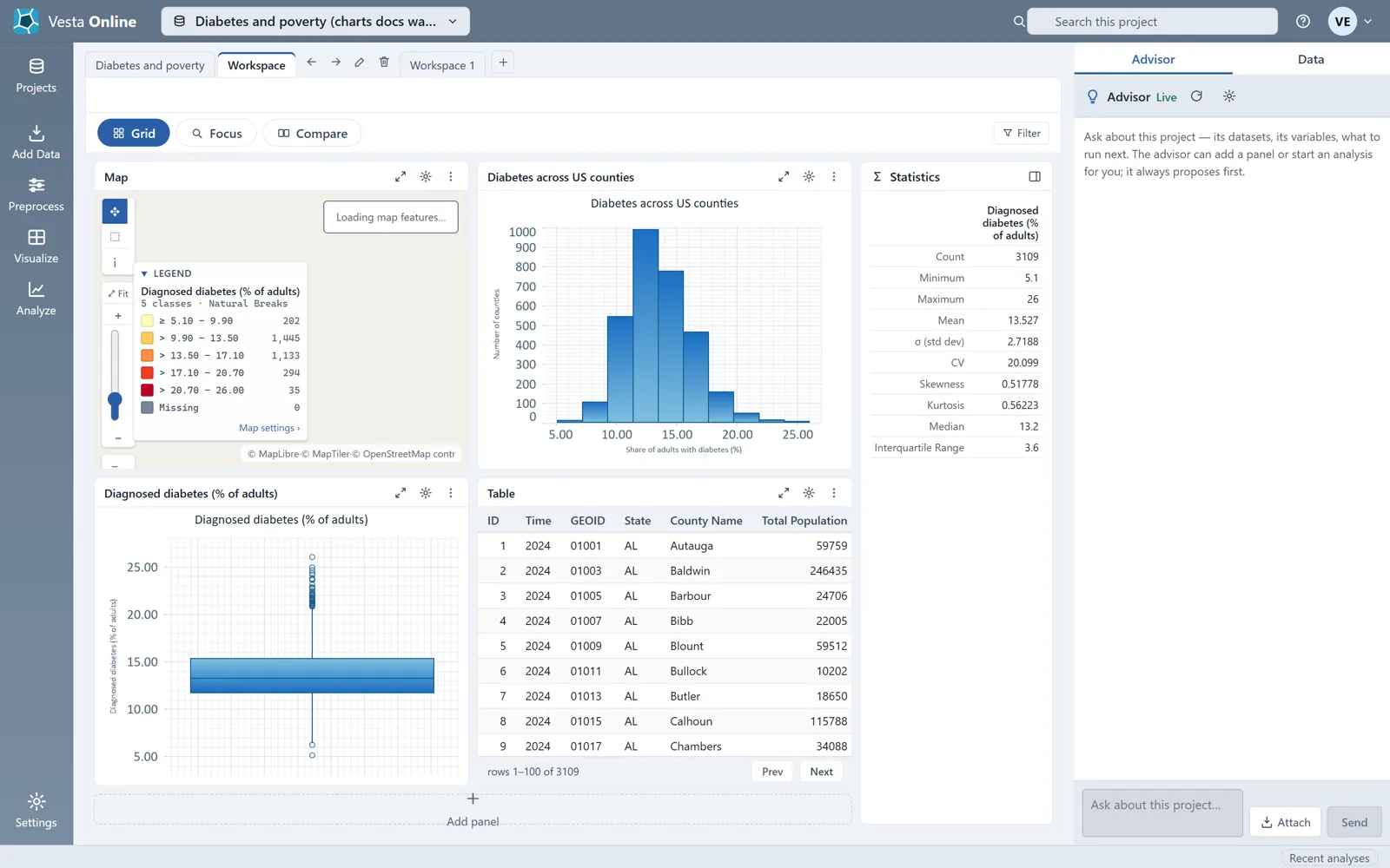
- Choose what you want to seeFour guided cards cover the common cases. Explore one variable ("Its distribution, spread, and geography.") builds a map, a histogram, a box plot and a table for the variable you pick. Compare two variables ("Maps side by side plus their relationship.") builds two maps, a scatter plot and a correlation matrix for variables A and B. Explore many variables ("Correlations and patterns across several at once.") is the third guided card. Show an analysis result ("Maps, plots, and summaries from a finished analysis.") builds panels from an analysis you have already run. Here, choose Explore one variable and pick Diagnosed diabetes (% of adults).
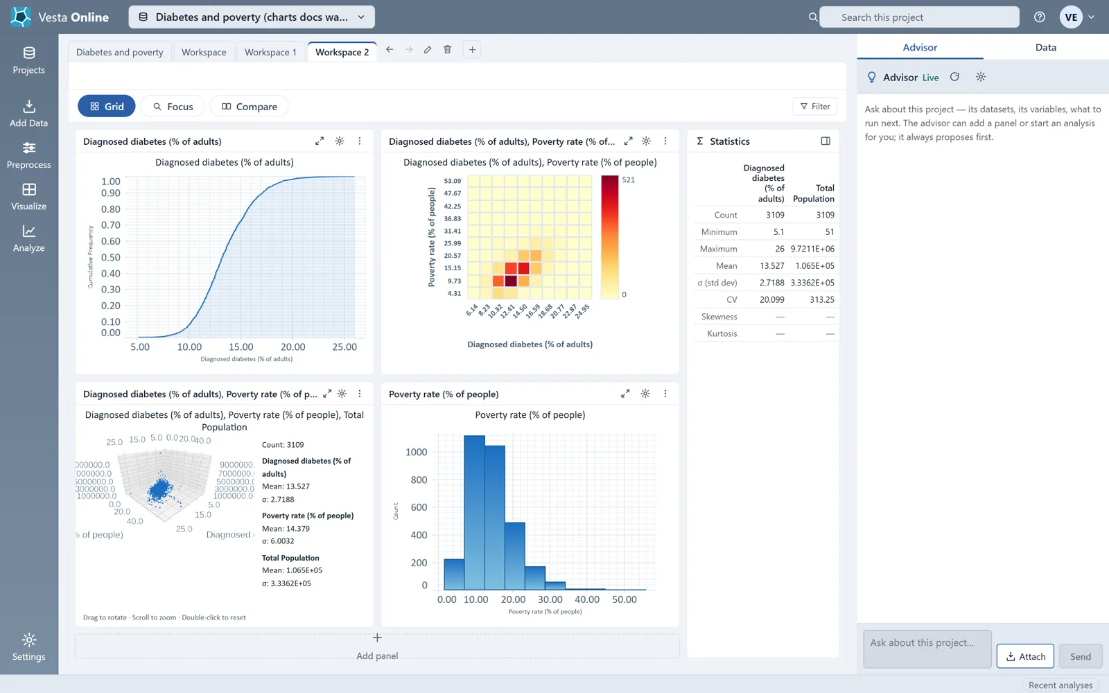
- Create the workspaceChoose Create workspace. Vesta adds a new workspace tab with the four panels from the preview. Each chart draws from your data, and a Statistics panel beside the grid lists the count, minimum, maximum, mean, standard deviation and more for the variable.
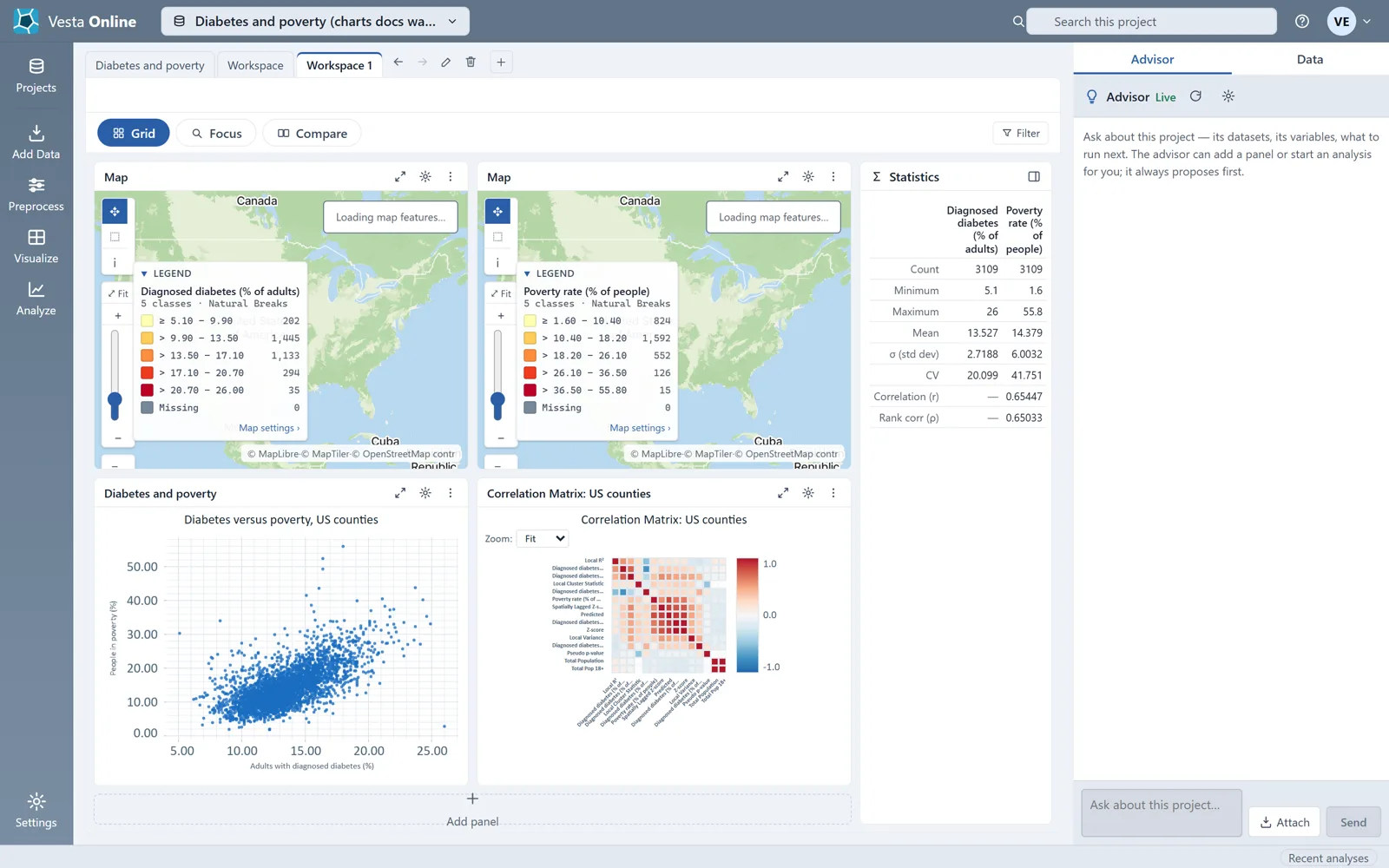
- Compare two variablesGo back to Visualize, choose Compare two variables, set A to Diagnosed diabetes (% of adults) and B to Poverty rate (% of people), and choose Create workspace. The scatter plot draws one point per county, and the Statistics panel adds the correlation (r) and the rank correlation (ρ) of the pair.
- Open the chart settingsChoose the gear in a chart panel's header. The Visualization settings dialog opens over the workspace. A map has its own Map settings instead.
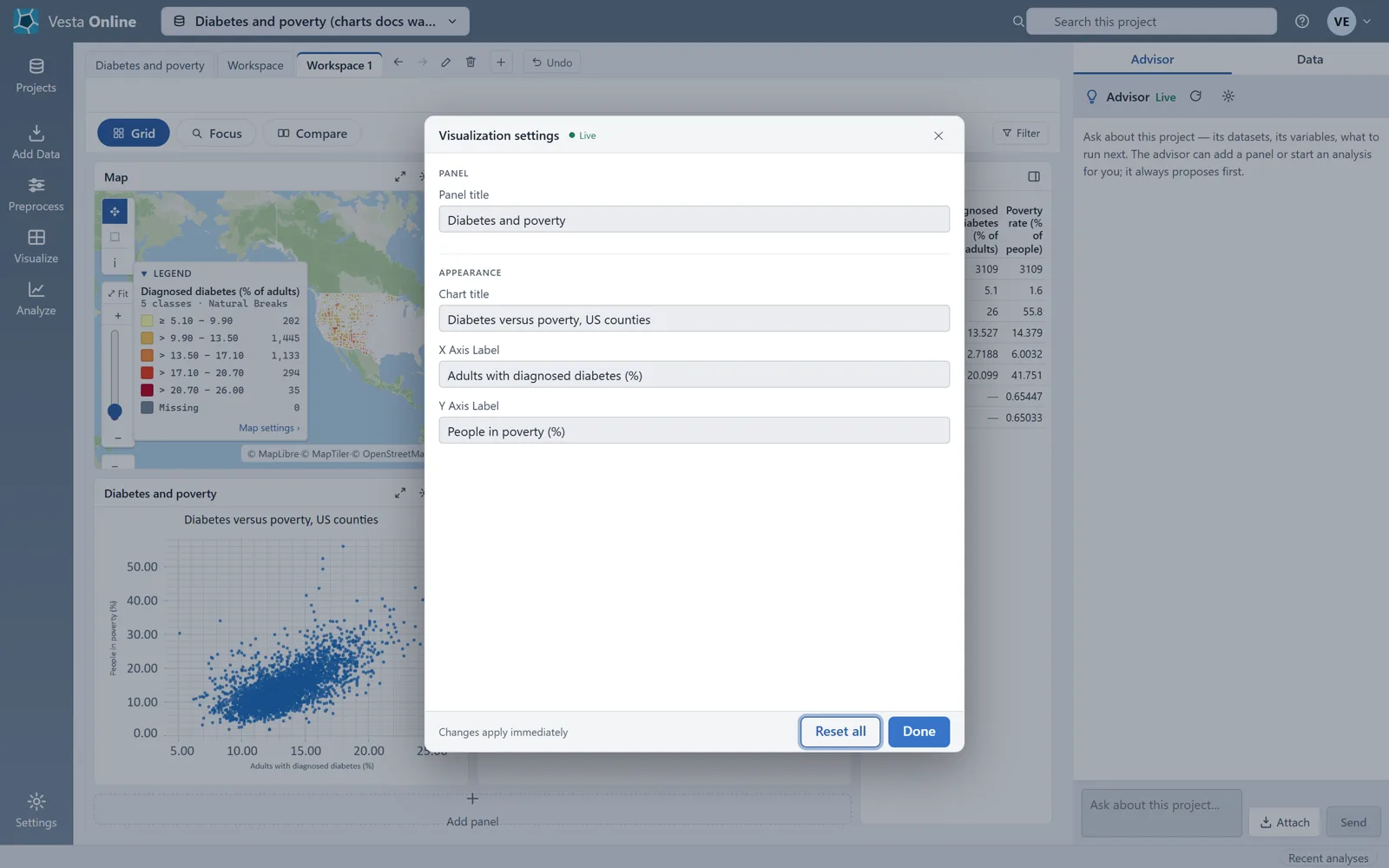
- Change the titles and labelsThe dialog has four boxes: Panel title, then under Appearance Chart title, X Axis Label and Y Axis Label. Type a new value in any of them. On the scatter plot used here, the walk typed all four values one after another, and the new title and labels showed in the panel without an apply step; the dialog is marked Changes apply immediately. The dialog also has Reset all.
- Close the settingsChoose Done, or press Escape. The chart keeps its new title and axis labels, and the workspace saves the change: after a reload the scatter plot still showed all three.
- Change a histogram's titles and labelsOpen the Explore one variable workspace again and choose the gear in the histogram's header. Its dialog has the same four boxes and a Bins section with Number of bins, here 10. Type a Chart title, an X Axis Label and a Y Axis Label, then choose Done. The histogram draws the new chart title and both axis labels, and they were still there after a reload.
- Build a workspace by handOn the hub, choose the Manual card ("Build the workspace yourself — layout and every panel."). Pick a layout with the four buttons: One panel, Two side by side, One large, two stacked, or Four panels. Choose a slot's header to open the catalog of views.
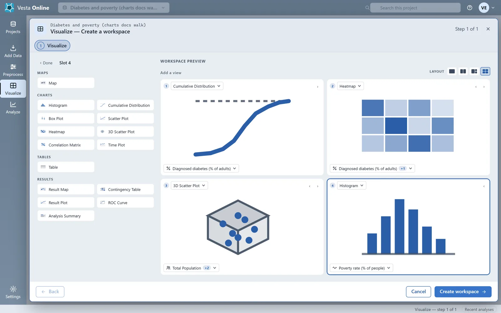
- Pick a chart type and its variables for each panelThe catalog groups views as Maps, Charts, Tables and Results. The Charts group lists Histogram, Cumulative Distribution, Box Plot, Scatter Plot, Heatmap, 3D Scatter Plot, Correlation Matrix and Time Plot. After you choose a type, pick its variables at the bottom of the slot: one variable for a histogram, cumulative distribution or box plot, two for a heatmap or scatter plot, three for a 3D scatter plot. This walk-through fills four slots with a cumulative distribution, a heatmap, a 3D scatter plot and a histogram, then chooses Create workspace.
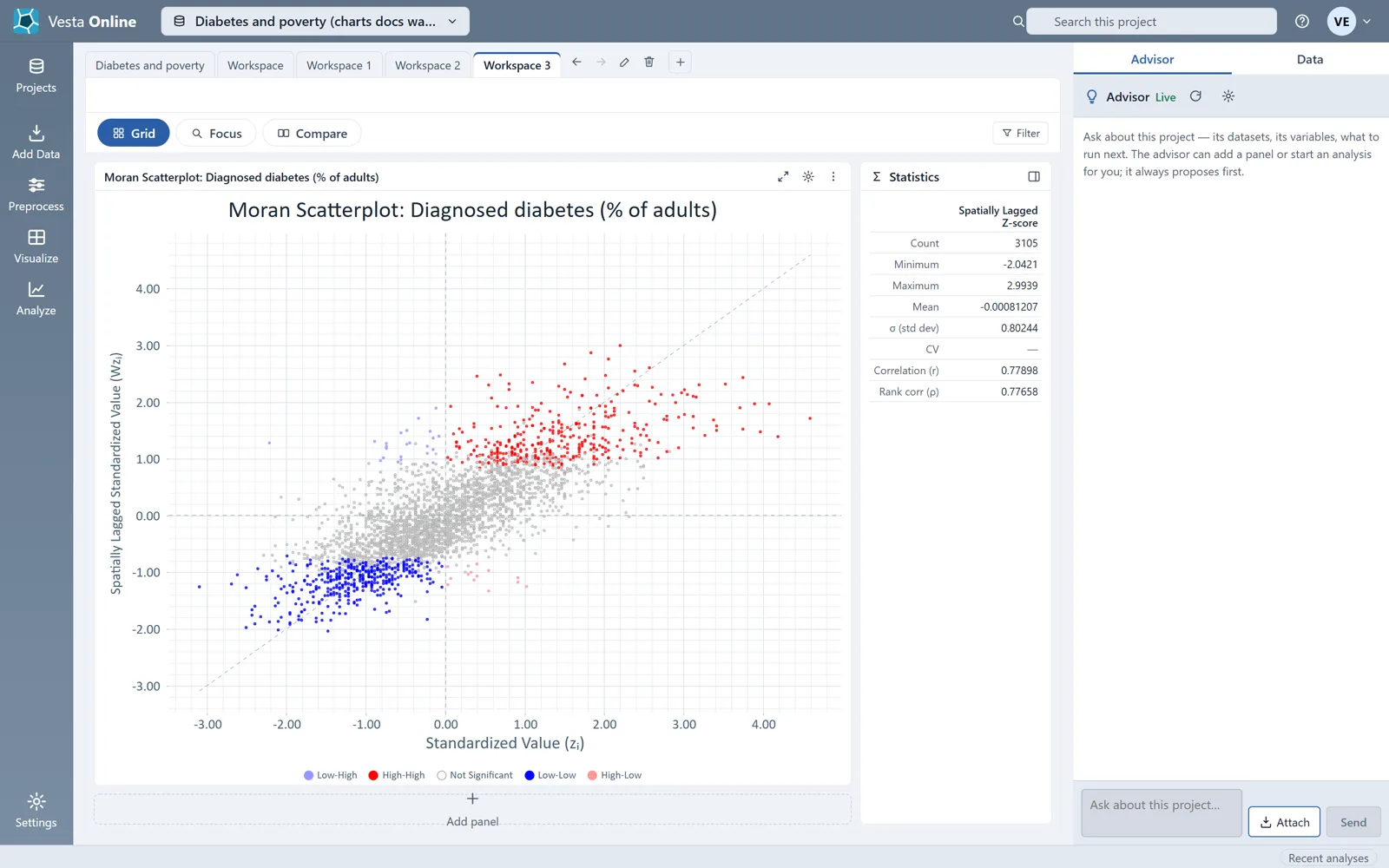
- Show an analysis resultChoose Show an analysis result and pick the analysis output from the list. The sample ships with a Local Cluster Analysis, so the list includes Moran Scatterplot. Choose it and Create workspace; the Moran scatterplot opens in its own workspace, colored by cluster class.
- Add a chart to a workspace you haveIn a workspace, choose Add panel under the grid. The hub opens with Create new and Adjust current, and its main button reads Update workspace. This walk-through opened the hub from Add panel and did not build a panel from it.
What you should see
Section titled “What you should see”The hub
Section titled “The hub”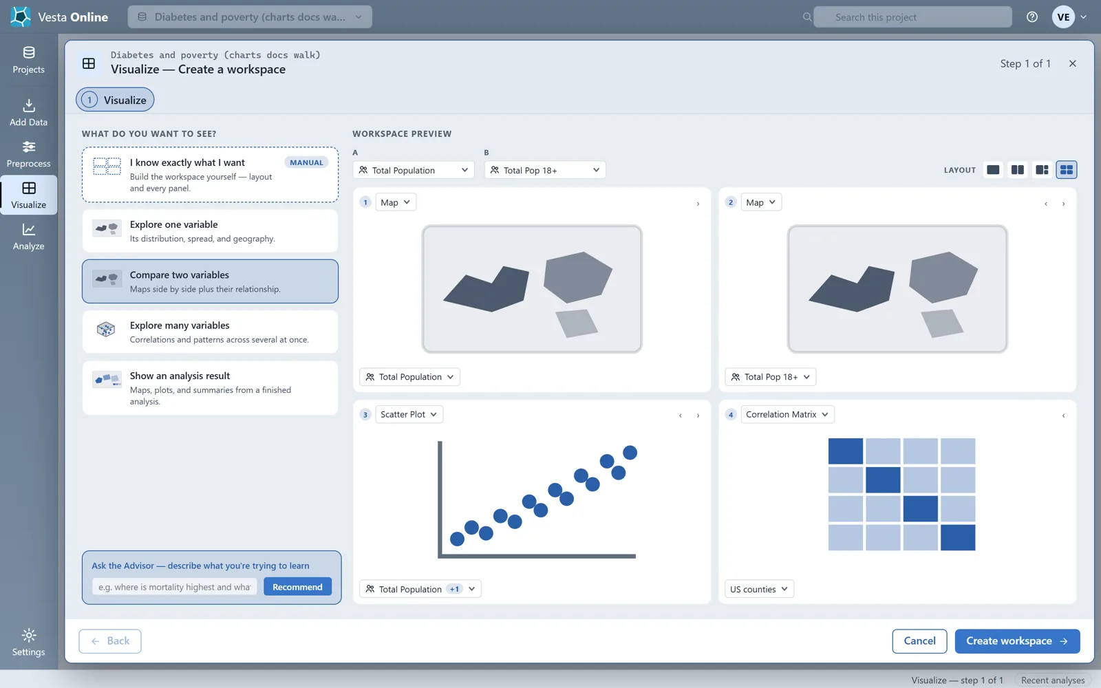
Explore one variable
Section titled “Explore one variable”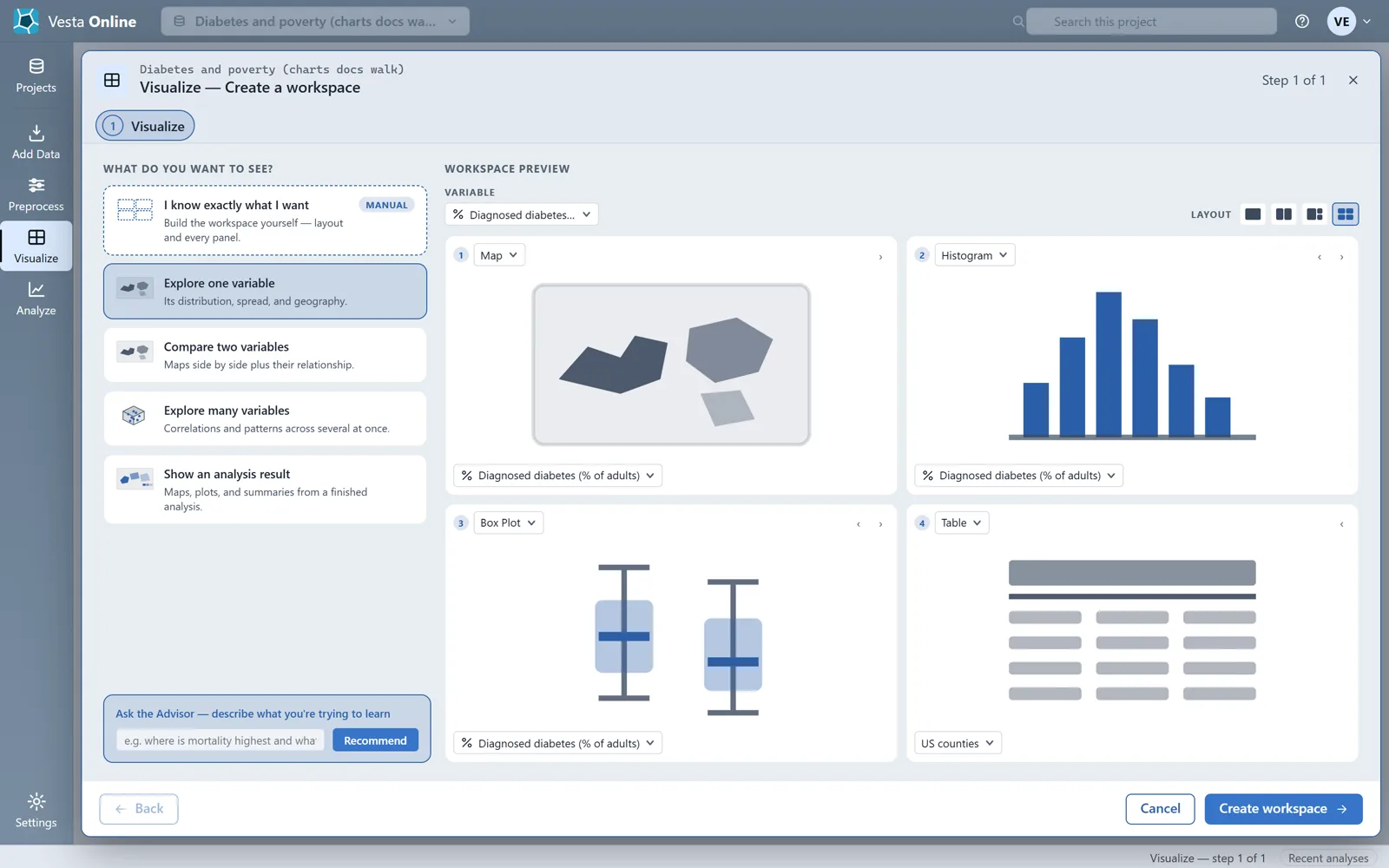
The workspace it creates
Section titled “The workspace it creates”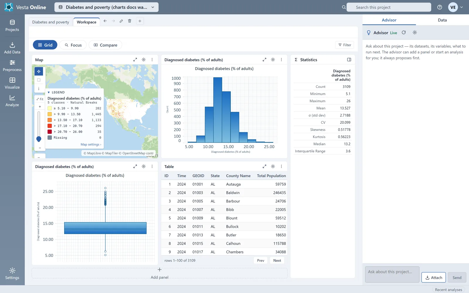
Compare two variables
Section titled “Compare two variables”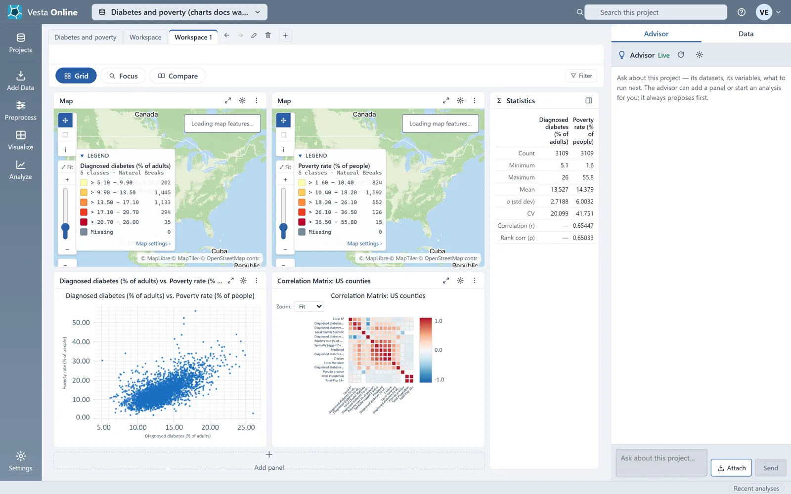
The settings dialog
Section titled “The settings dialog”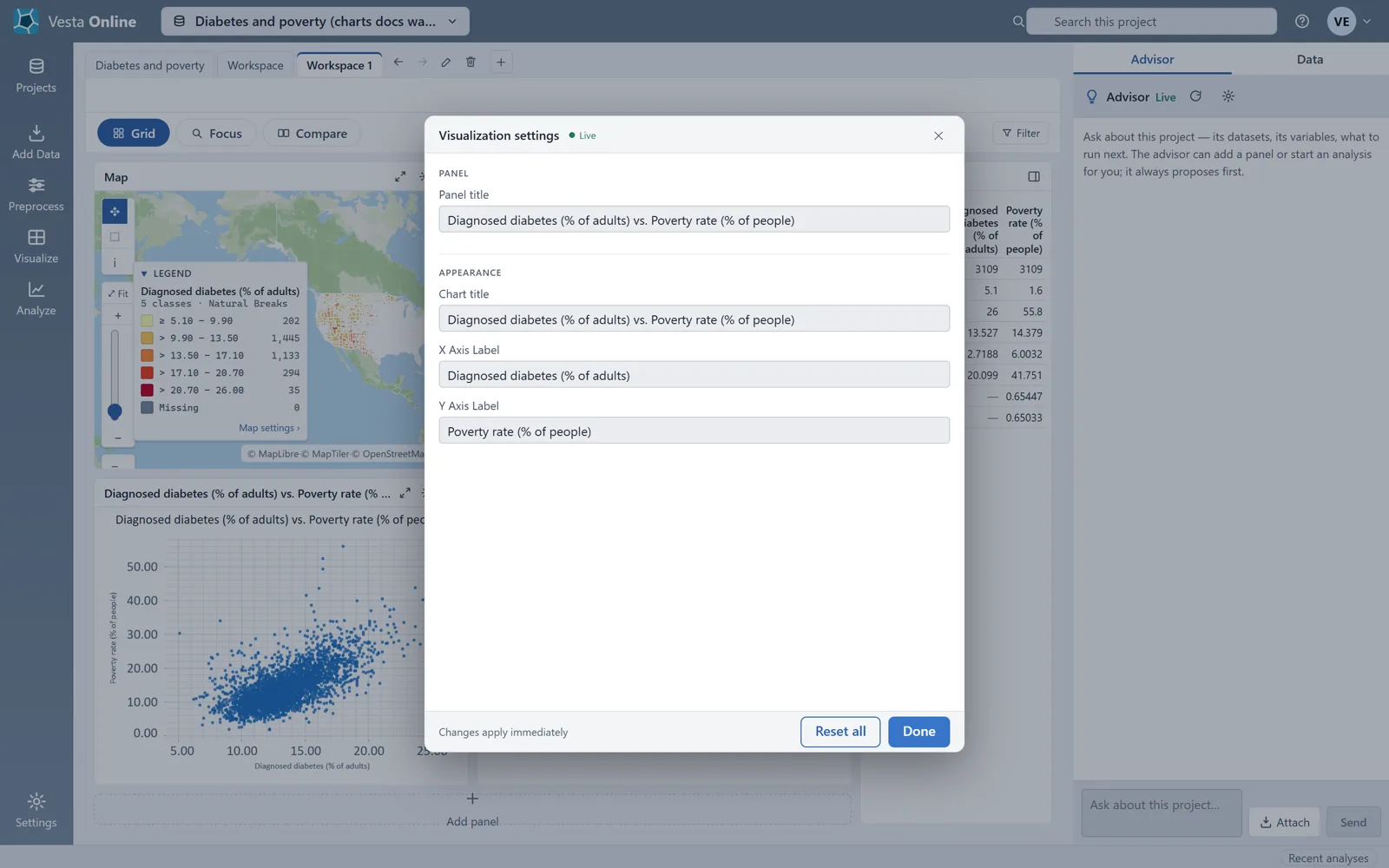
The manual catalog
Section titled “The manual catalog”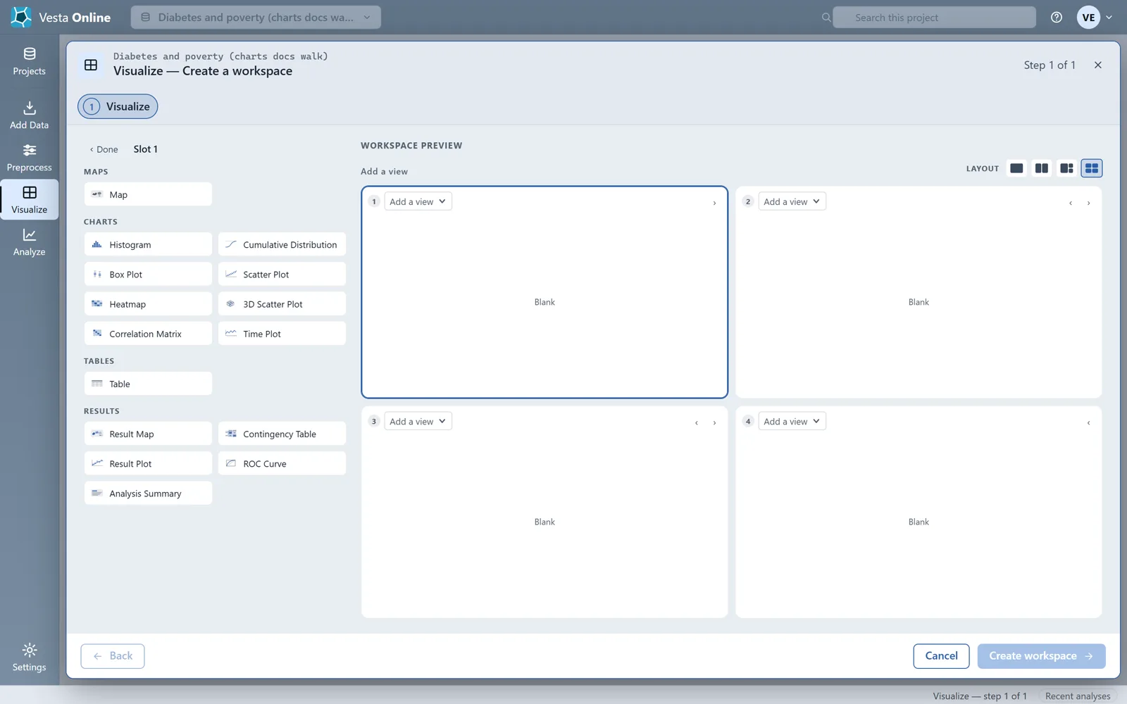
The Moran scatterplot
Section titled “The Moran scatterplot”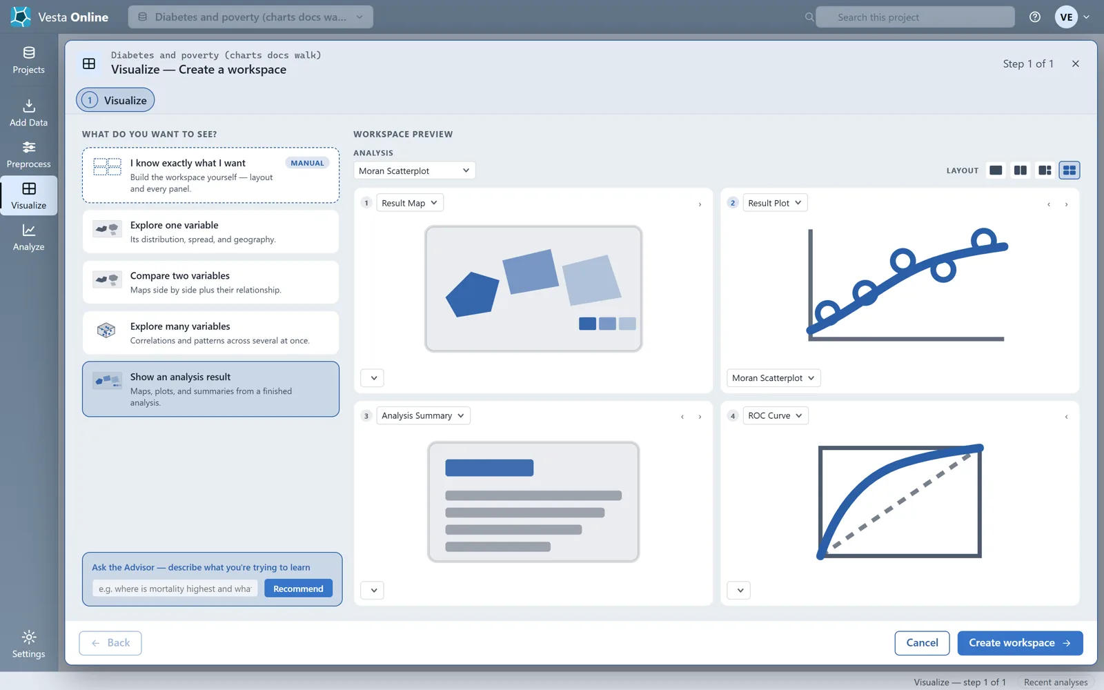
Add panel
Section titled “Add panel”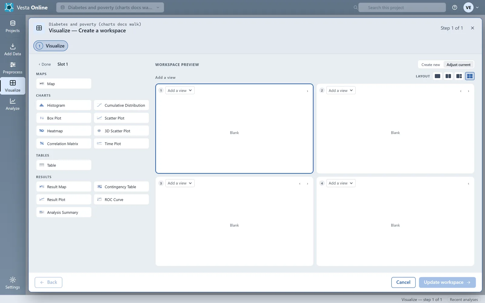
Reading the charts
Section titled “Reading the charts”| Chart | Variables you pick | Where it appeared in the walk |
|---|---|---|
| Histogram | One | Explore one variable; the manual workspace |
| Cumulative Distribution | One | The manual workspace |
| Box Plot | One | Explore one variable |
| Scatter Plot | Two | Compare two variables |
| Heatmap | Two | The manual workspace |
| 3D Scatter Plot | Three | The manual workspace |
| Correlation Matrix | Not picked in the walk | Compare two variables |
| Time Plot | Not walked | Not walked |
The Moran scatterplot is the scatter plot a Local Cluster Analysis saves. Its chart title starts with “Moran Scatterplot: “ followed by the variable name, and the points are colored by cluster class. To make one, run the analysis as described in Local cluster analysis and choose it under Show an analysis result.
Where next
Section titled “Where next”- How panels, tabs and layouts work: The workspace.
- Make the result behind the Moran scatterplot: Local cluster analysis.
- Work on a map next to the chart: Maps.