Variography
Fit a variogram model in Vesta Online: choose the variable, build the experimental variogram, let Vesta fit the model, save it and reuse it in kriging.
Variography measures how a variable’s similarity decays with distance and fits a model to that decay. The fitted model, a variogram, is what kriging uses to weight observations. This walk-through uses the Well-water arsenic sample (186 wells), copied into a new project. It fits a variogram to the arsenic values with the defaults at the Guided level, saves it, reads the result and then picks the saved model in kriging. It also sets the model by hand, adds a leave-one-out cross-validation and switches anisotropy on at Full control, then restores Auto-fit and turns anisotropy off before saving. Other options (the Automatic guidance level, a Trend, the Indicator and Compositional value types and Manual lag mode) are described from Vesta’s own text and were not walked.
The steps
Section titled “The steps”- Open the sample projectOpen a project that holds your point data. This walk uses a copy of the Well-water arsenic sample, so the sample itself stays untouched. Its dataset Salt Lake County wells has 186 wells.
- Choose VariographyChoose Analyze, then Describe spatial structure, then Variography. The flow has seven steps: Analysis, Variable, Experimental, Model, Anisotropy, Save and Summary.
- Choose the dataset and the variableUnder Dataset choose Salt Lake County wells, and under Variable choose Arsenic (µg/L). Leave the value type on Continuous. Choose Next: Experimental.
- Set the lagsOn Experimental, leave the estimator on Traditional and the lag count at 20. The plot beside the settings shows the experimental points, the fitted curve and a dashed line for the sample variance, and refits as you change a setting.
- Choose the modelOn Model, leave the family on Auto, which tries Spherical, Exponential and Cubic and keeps the best fit. Leave Nested structures at 2. The model is saved under the name in Variogram name, by default the variable's name followed by Variogram.
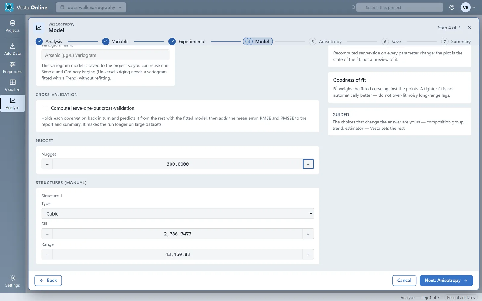
- Or set the model by handTo set the fit yourself, clear Auto-fit model, sills & ranges on Model. At Guided, the default level, the Nugget field and one card per structure, with its type, sill and range, appear, starting from the last fit, and the fit numbers beside the plot follow what you enter. This walk sets the nugget to 300.
- Turn auto-fit back onTick Auto-fit model, sills & ranges again. The hand-set nugget no longer shows beside the plot.
- Add a cross-validationTo check the fitted model against the data, tick Compute leave-one-out cross-validation on Model. Vesta holds each observation back in turn, predicts it from the rest with the fitted model and adds the mean error, RMSE and RMSSE to the report and summary. It makes the run longer on large datasets. This walk leaves it ticked through the save.
- Check for anisotropyOn Anisotropy, leave Include anisotropy off for one range in every direction. This walk leaves it off first.
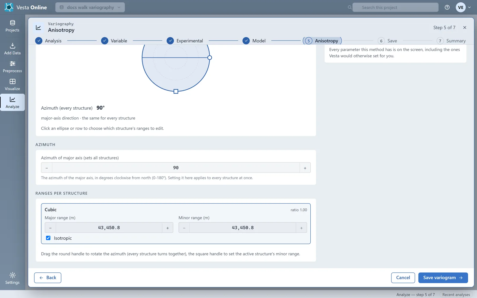
- Or turn anisotropy onTick Include anisotropy and raise the guidance level to Full control. Lags & bins and a Specification appear. Auto-detect fits the direction and ranges from the data and reports what it detected, with a confidence and a direction; here it reports no significant anisotropy. Choose Manual to enter the azimuth of the major axis, one value for every structure, and each structure's major and minor ranges, or drag the round handle on the ellipse to set the azimuth; dragging it due east set the Azimuth field near 90. With anisotropy on, the plot shows the experimental points in four directions.
- Turn anisotropy off againClear Include anisotropy and return the guidance level to Guided before you save.
- Save the variogramChoose Save variogram. The fit runs on the server, and the Summary step lists what was saved: the variogram model, a report and an analysis summary, plus the cross-validation results when Compute leave-one-out cross-validation is ticked.
- Open the result workspaceChoose Open in workspace. The result workspace opens with the analysis summary, the variogram plot, the variogram map and the fit summary.
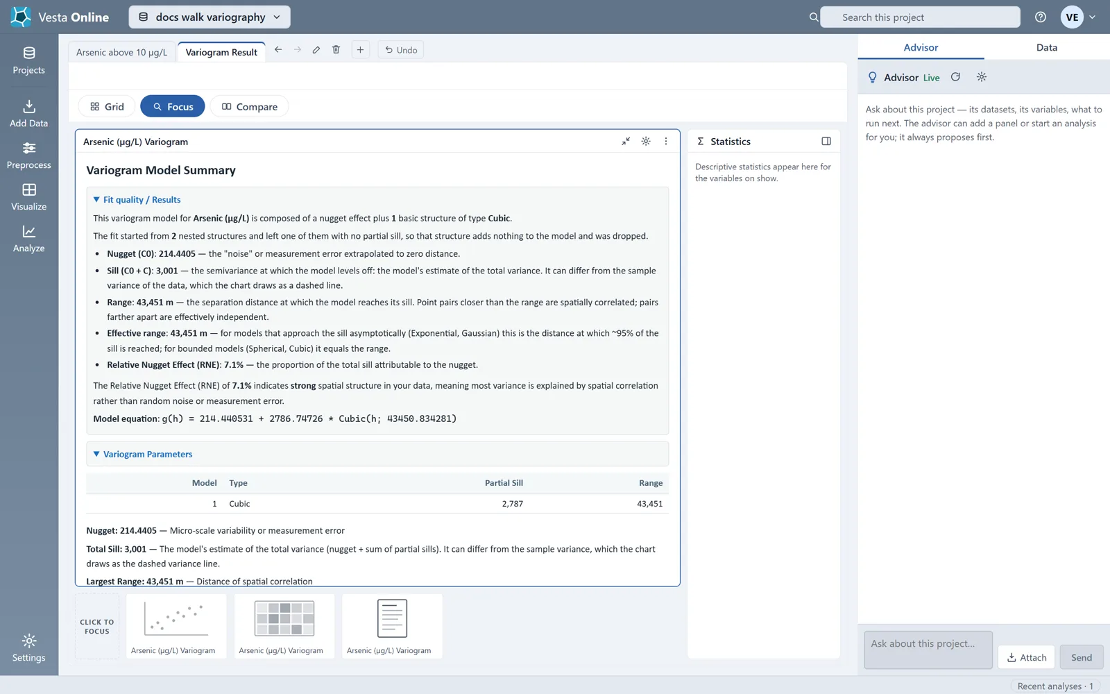
- Read the summaryUse Focus on the summary panel to read it full width. It describes the fitted model, its parameters and the relative nugget effect.
- Use the model in krigingStart Kriging, choose the same variable and, on the Variogram step, choose Use a saved model. Pick the saved model from the Variogram model list. Kriging reuses it without refitting.
What you should see
Section titled “What you should see”The variable
Section titled “The variable”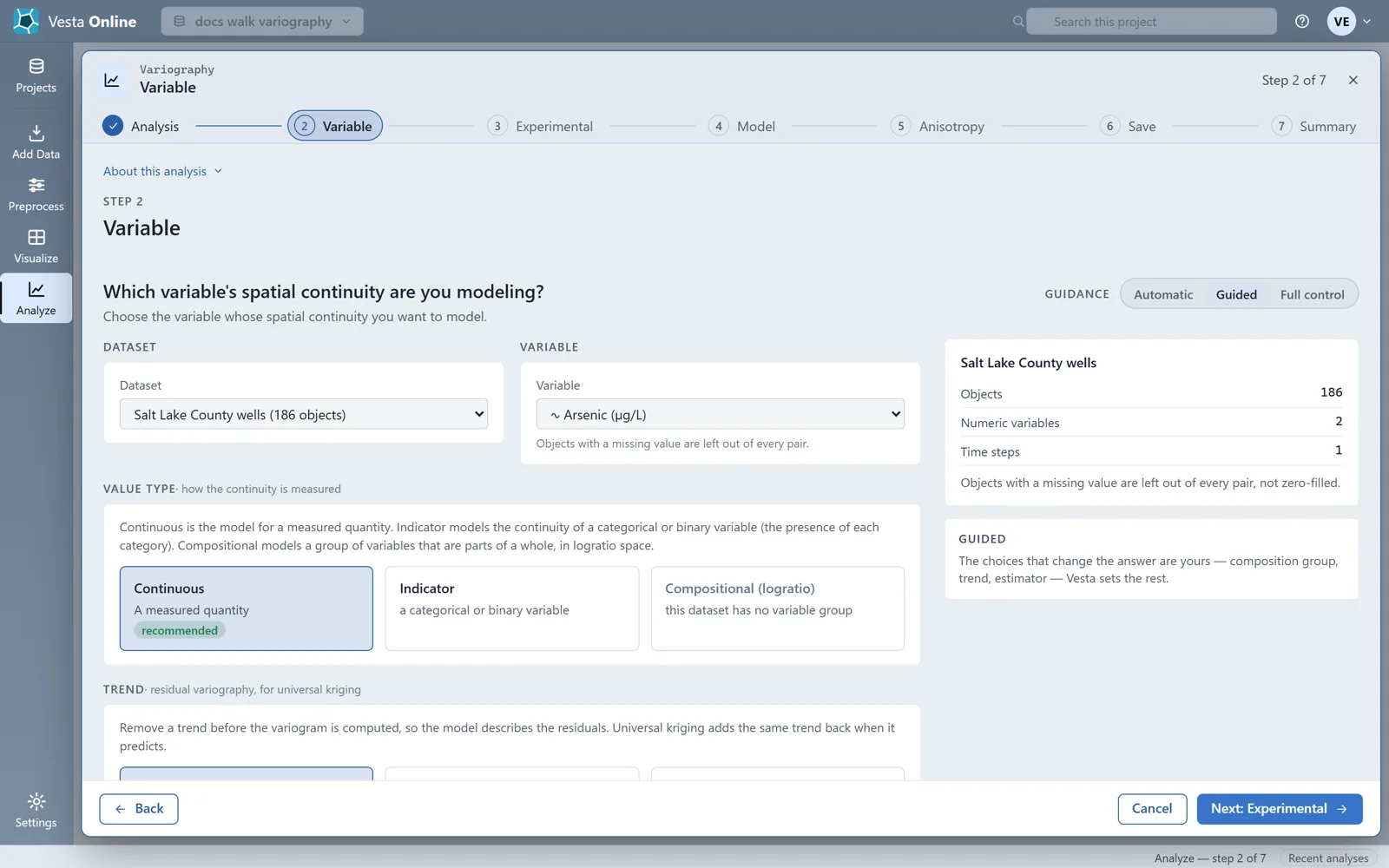
Objects with a missing value are left out of every pair, not zero-filled. The value type sets how continuity is measured:
| Value type | What it models |
|---|---|
| Continuous | A measured quantity, such as a concentration. |
| Indicator | The continuity of a categorical or binary variable: the presence of each category. |
| Compositional (logratio) | A group of variables that are parts of a whole, modeled together in logratio space. It needs a variable group in the dataset. |
The Trend choice, below the value type, is for universal kriging. With a trend chosen, Vesta removes the trend before the variogram is computed, so the model describes the residuals, and universal kriging adds the same trend back when it predicts.
The experimental variogram
Section titled “The experimental variogram”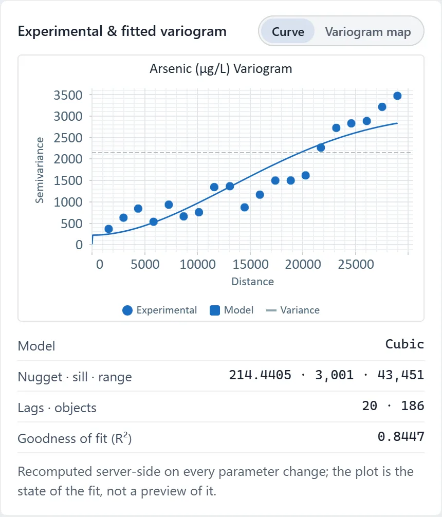
Each point is one lag bin: the mean semivariance of every pair whose distance falls in it. Long-range lags carry few pairs and are the noisiest, so they should not drive the fit. The estimators include Traditional, Standardized and Weighted; Weighted needs a weight variable. The plot is recomputed on the server on every change, so it shows the current fit, not a preview of it.
By default Vesta chooses the lag width from the extent of the data; the lag width becomes a control when you raise the guidance level to Full control. The Spatio-temporal option turns the variogram into a space-time surface, with both plots in 3D over spatial and temporal lag. It needs data at more than one time: the wells carry a single time, so it cannot be used here.
The model
Section titled “The model”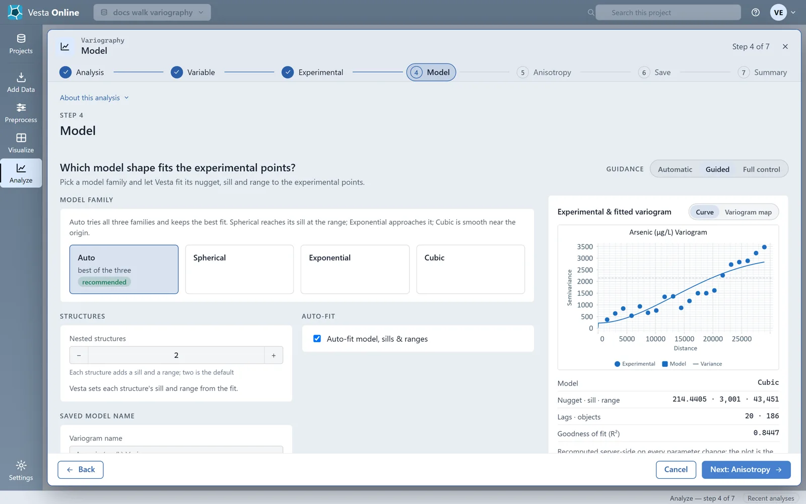
Spherical reaches its sill at the range, Exponential approaches it, and Cubic is smooth near the origin. Each nested structure adds a sill and a range. Vesta sets each structure’s partial sill and range from the fit. R-squared weighs the fitted curve against the points; a tighter fit is not automatically better, so do not over-fit noisy long-range lags.
With Auto-fit model, sills & ranges ticked, Vesta fits the nugget and each structure’s sill and range. Clearing the box overrides that fit: a Nugget field and a card per structure, with Type, Sill and Range, appear, starting from the last fit, and the model uses the values you enter. The walk showed these fields at Guided, the default level.
Cross-validation
Section titled “Cross-validation”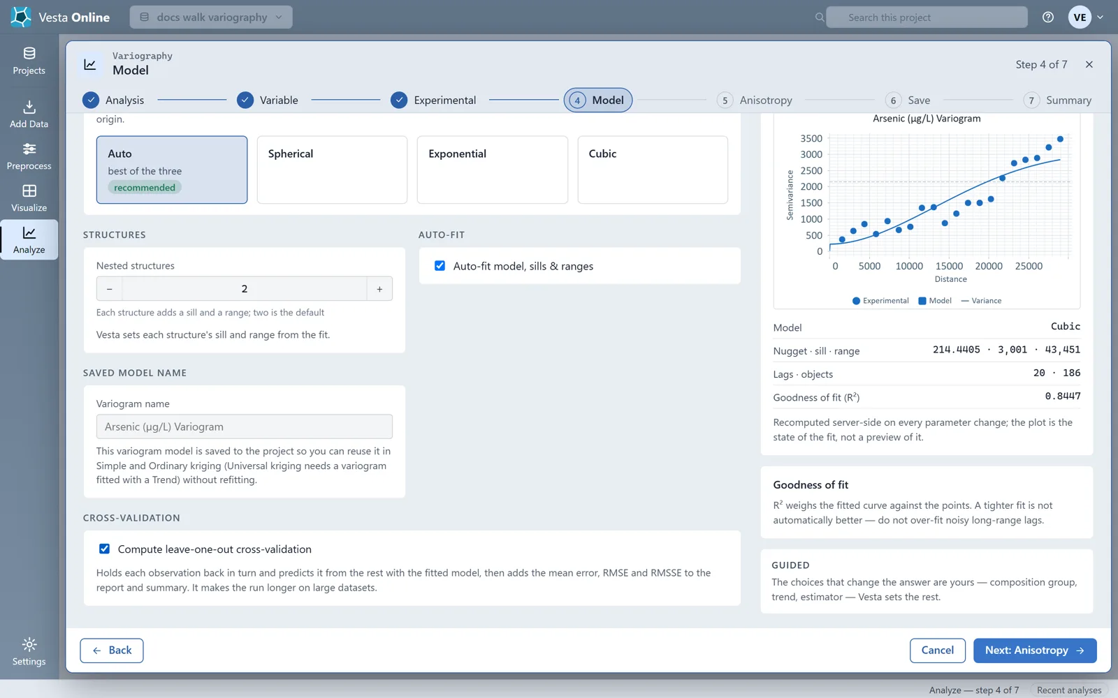
Leave-one-out cross-validation holds each observation back in turn and predicts it from the rest with the fitted model, then adds the mean error, RMSE and RMSSE to the report and summary. It makes the run longer on large datasets. It is not available for a space-time model, a compositional model or a cross-variogram, and the box says so when that is the case. On the arsenic wells it reported a mean error of -0.216, an RMSE of 41.959 and an RMSSE of 0.908. Read them as the summary does: the mean error should be close to 0, a smaller RMSE is better, and an RMSSE near 1 means the model states its uncertainty about right. The Summary step lists the cross-validation among what was saved.
Anisotropy
Section titled “Anisotropy”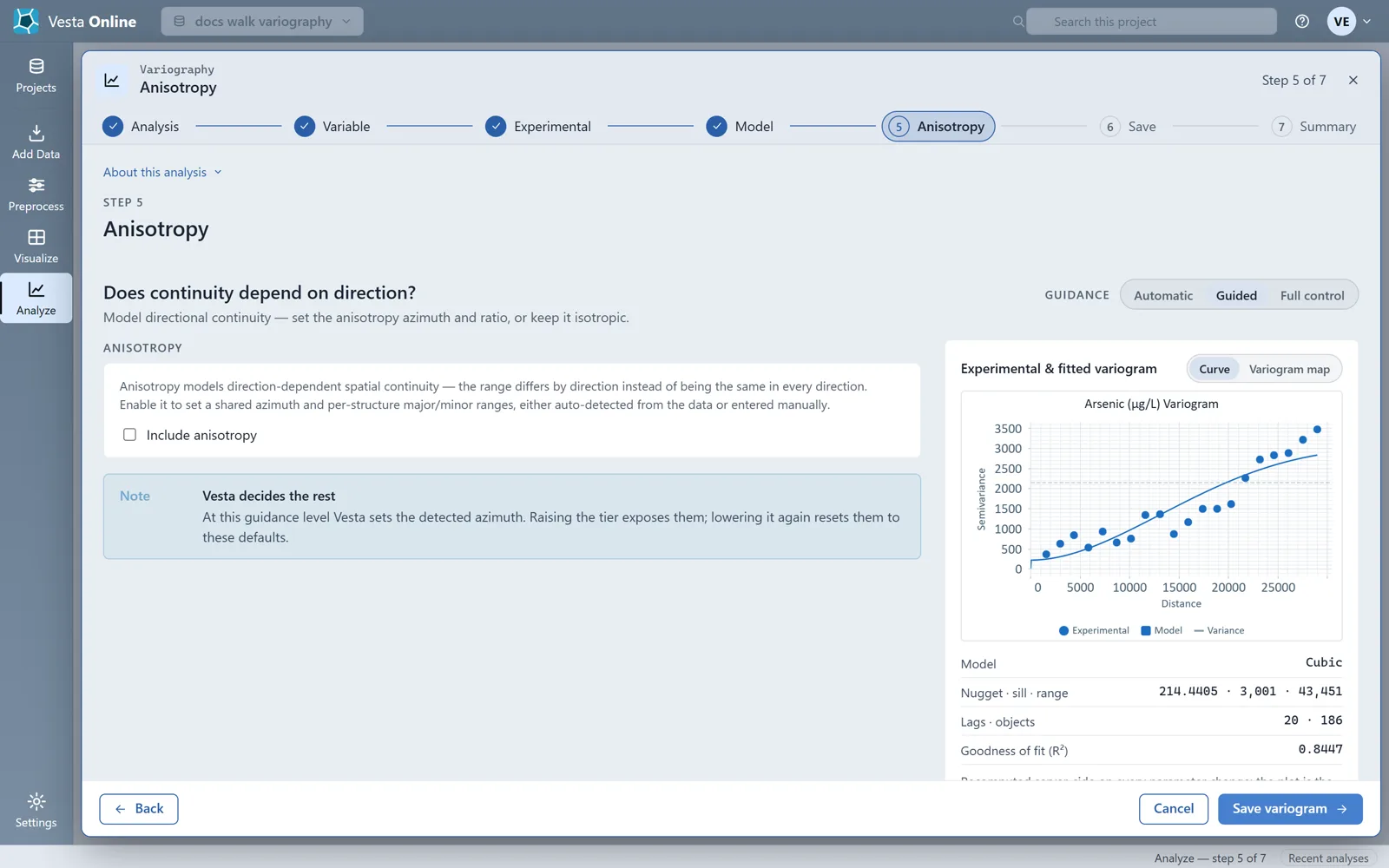
With anisotropy on, the step adds Lags & bins and, at Full control, a Specification, and the pairs are split across four directions. Auto-detect detects the direction during the fit and shows a Detected card with a confidence and a direction; Re-detect anisotropy from data refits. In this run it reported a confidence of 0% and no significant anisotropy. Manual gives you the Azimuth of major axis, in degrees clockwise from north (0 to 180), and a major and a minor range for each structure.
Saving
Section titled “Saving”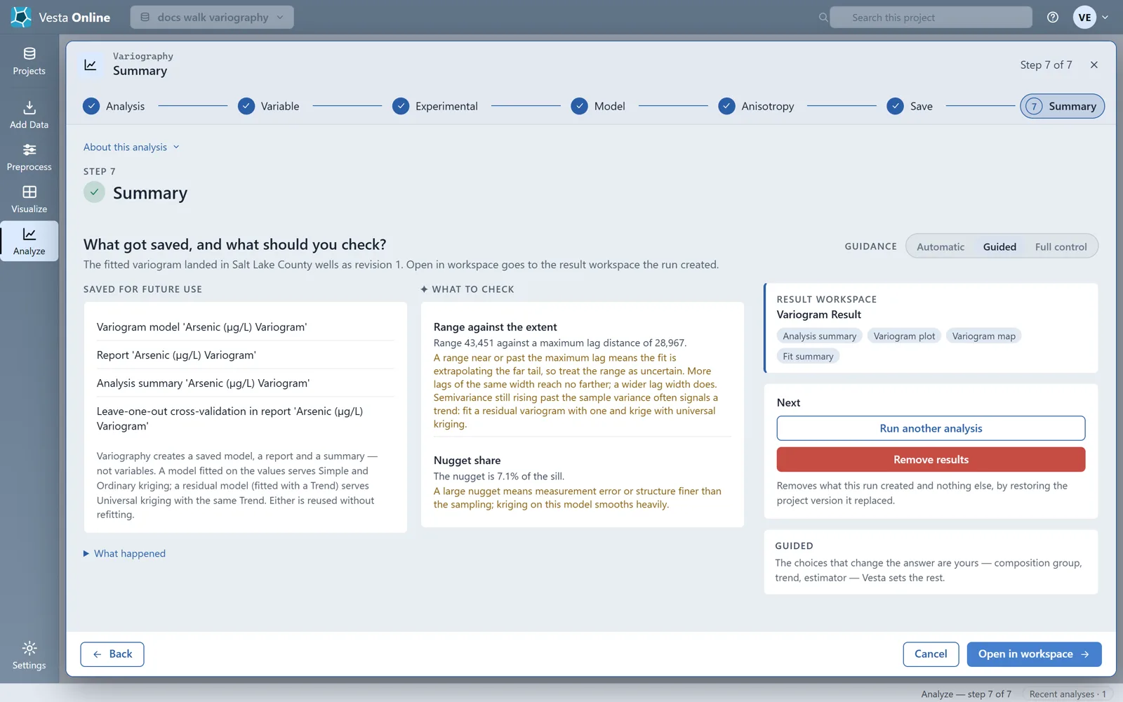
Variography creates a saved model, a report and a summary, not variables. A model fitted on the values serves Simple and Ordinary kriging; a residual model, fitted with a trend, serves universal kriging with the same trend. Either is reused without refitting.
The What to check cards flag the two things to look at first. In this run, the range of 43,451 is larger than the maximum lag distance of 28,967, which means the fit is extrapolating the far tail. The nugget is 7.1% of the sill.
Remove results removes what this run created and nothing else, by restoring the project version it replaced. Only one analysis of yours runs at a time: if another is still running when you save, the step says so, and you can try again when it has finished.
The result workspace
Section titled “The result workspace”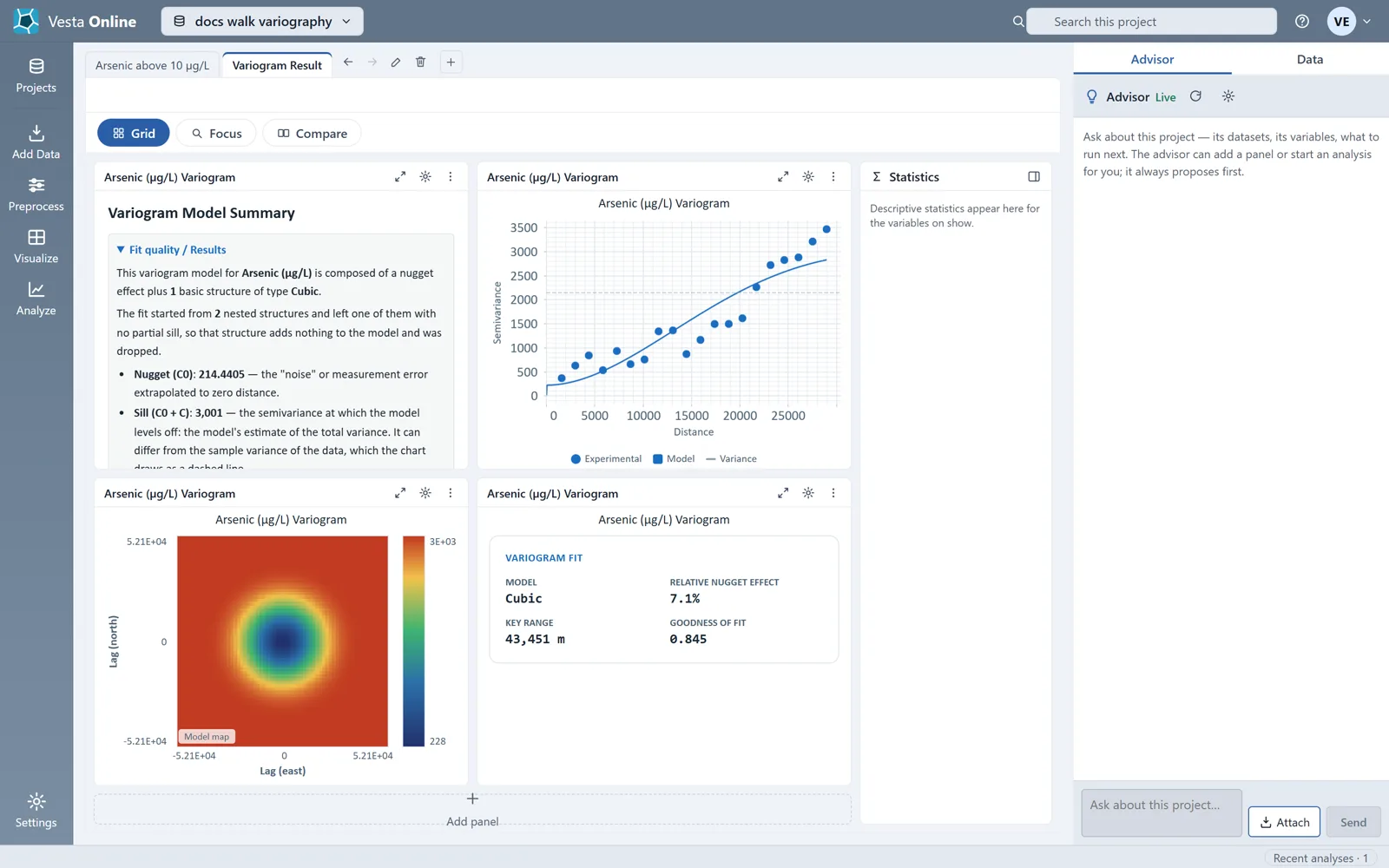
Reading the results
Section titled “Reading the results”| Parameter | What it means |
|---|---|
| Nugget | Variation at zero distance: measurement error, or structure finer than the sampling. |
| Sill | The level at which the model levels off: the nugget plus every partial sill. It is the model's estimate of the total variance. |
| Range | The distance at which the model reaches its sill. Pairs closer than the range are spatially correlated; pairs farther apart are effectively independent. For Exponential, use the effective range. |
| Effective range | For models that approach the sill gradually (Exponential), the distance at which about 95% of the sill is reached. For Spherical and Cubic it equals the range. |
| Relative nugget effect (RNE) | The share of the total sill that comes from the nugget. |
The sill is fitted to the experimental points, so it can differ from the sample variance, which the plot draws as the dashed Variance line. In this run the sill is 3,001 and the dashed line sits near 2,150. The semivariance is still rising at the largest lag, well above the dashed line, so the fitted range lies beyond the data and the fitted sill sits above the sample variance. Semivariance that keeps climbing past the sample variance often signals a trend; if one is plausible, fit a residual variogram with a Trend and use universal kriging.
When the fit leaves a structure with no partial sill, that structure adds nothing to the model, so Vesta drops it and the summary says so. This run started from 2 nested structures and kept 1.
| RNE | What it indicates |
|---|---|
| Below 25% | Strong spatial structure: most variance is explained by spatial correlation rather than random noise or measurement error. |
| 25% to 75% | Moderate spatial dependence: a mix of spatially structured signal and unstructured noise. |
| Above 75% | Weak spatial dependence: most variability is micro-scale heterogeneity or measurement error. |
A large nugget means measurement error or structure finer than the sampling, and kriging on such a model smooths heavily. A range near or past the maximum lag means the fit is extrapolating the far tail, so treat the range as uncertain; at Full control you can set a wider lag width.
Using the model in kriging
Section titled “Using the model in kriging”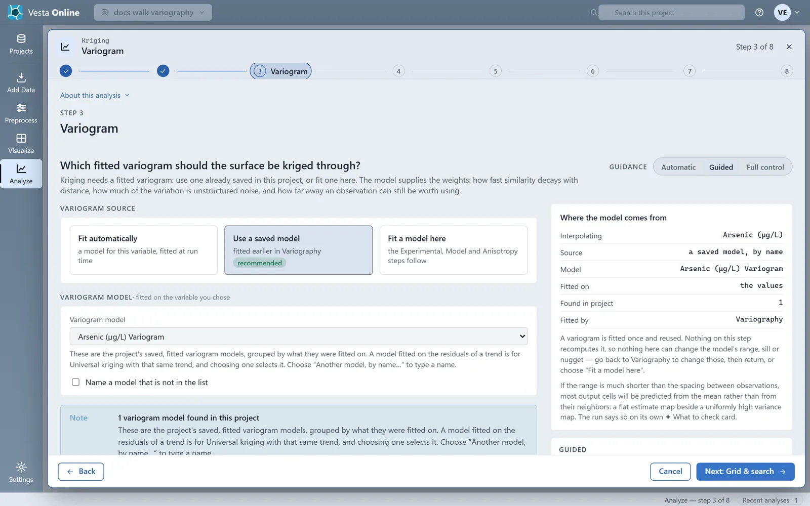
A variogram is fitted once and reused. Nothing on the kriging Variogram step recomputes it, so to change its range, sill or nugget, go back to Variography, or choose Fit a model here, which fits one inside the kriging run. See Kriging for the rest of that flow.
Where next
Section titled “Where next”- Interpolate with the saved model: Kriging.
- Run the full path from import to result: Quickstart.