Quickstart
Create a project, bring in county health data from the online catalog, map it and run a Local Cluster Analysis in Vesta Online.
This walk-through takes one public dataset from the online catalog to a map of statistically significant clusters: diabetes prevalence for Michigan counties from CDC PLACES. Every step below was run on Vesta Online; the screenshots come from that run.
The seven steps
Section titled “The seven steps”- Create a projectOpen the Projects page and choose New Project. Type a name in the Project name box and choose Create. The new project is selected in the list, ready to open.
- Add data from an online sourceChoose Open Project, then Add Data in the left rail. Under From an online source, choose the US Public Health category, then CDC PLACES. Vesta Online fetches from a curated catalog of public sources.
- Choose what to importChoose Next: Geography. Leave Geographic level on County and pick Michigan under States (leave States empty for the whole country). On Measures pick Diabetes, on Releases pick 2023, then choose Next: Review to check your choices.
- Run the importChoose Run import. The fetch runs on the server, so stay on the page until the Summary appears; it reports how many records landed in the new CDC PLACES dataset.
- Map the dataChoose Finish — open the project, then Visualize in the left rail. Choose Explore one variable, set the variable to Diabetes and choose Create workspace. The workspace opens with a map of Diabetes, its legend, and charts and a table beside it.
- Run a local cluster analysisChoose Analyze, then Find clusters & hotspots, then Local Cluster Analysis. On Variables choose Diabetes. On Spatial weights leave the neighbor definition on Detect. On Significance the defaults are an alpha of 0.05 and 100 randomizations. Choose Run analysis.
- Open the result workspaceWhen the Summary says what was saved, choose Open in workspace. The result workspace shows the cluster map, a category counts histogram, a Moran scatterplot and the analysis summary.
What you should see
Section titled “What you should see”A new project
Section titled “A new project”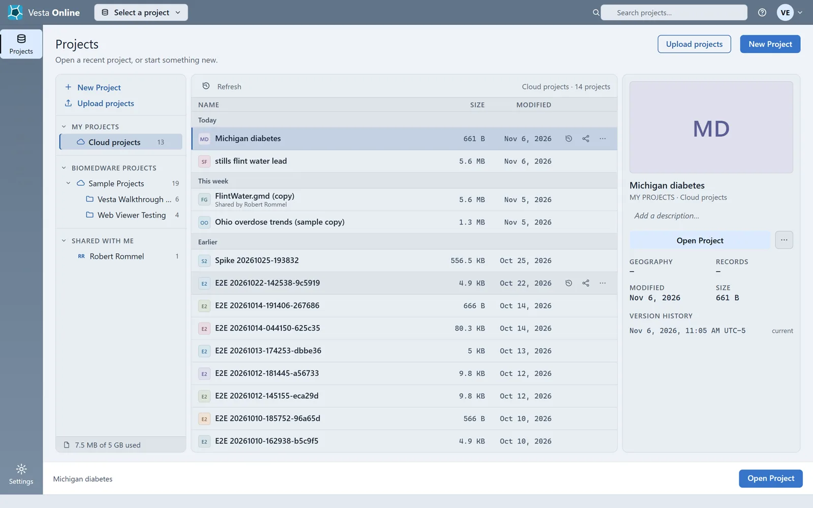
The catalog
Section titled “The catalog”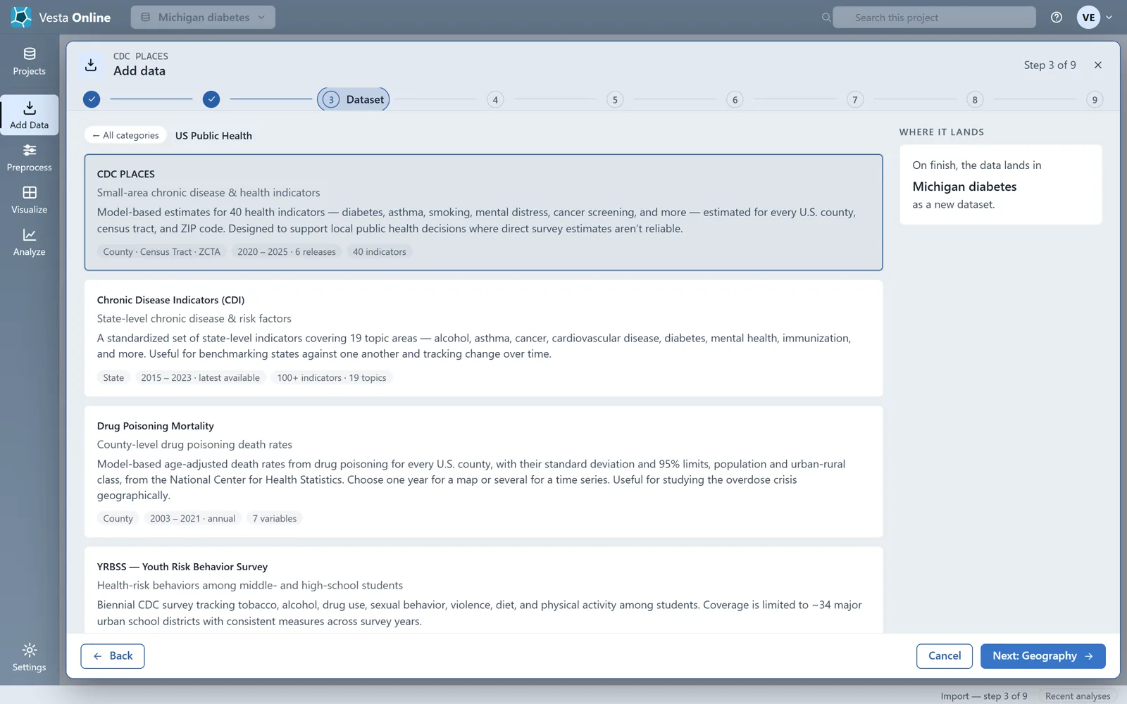
The import review
Section titled “The import review”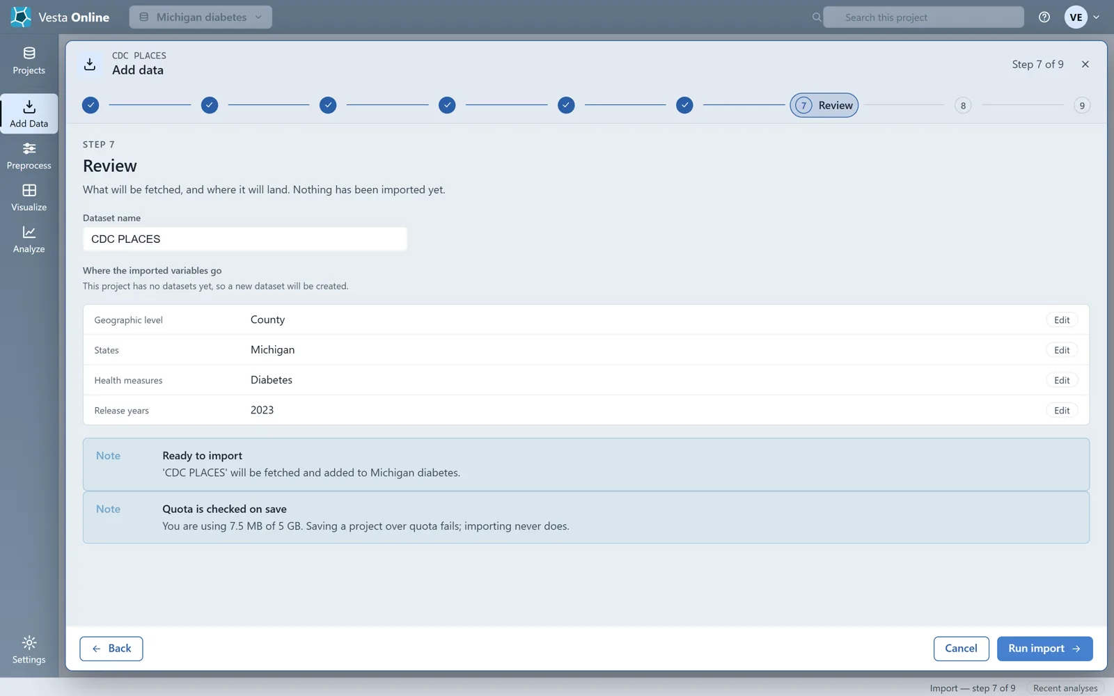
The import summary
Section titled “The import summary”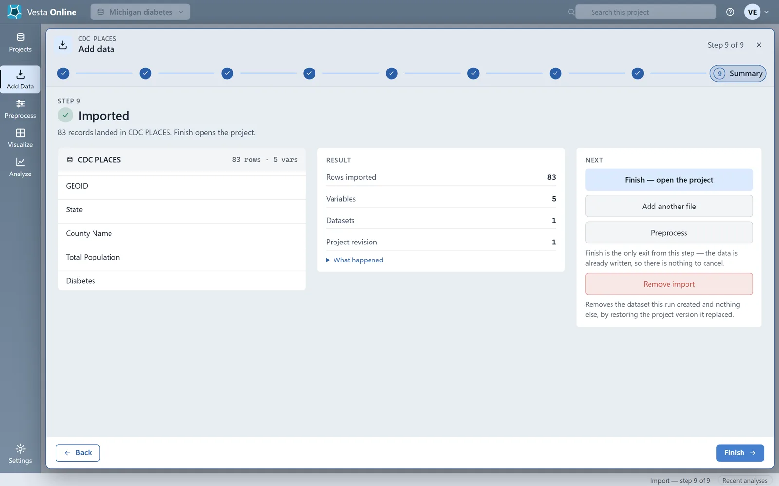
The map
Section titled “The map”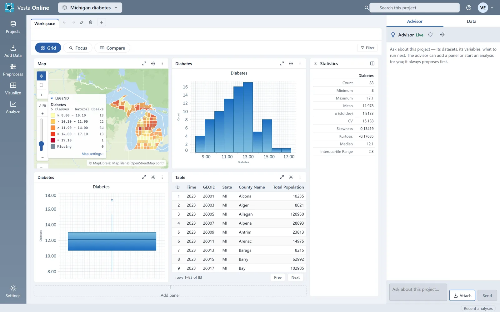
The analysis
Section titled “The analysis”Local Cluster Analysis compares each county’s value with its neighbors’ and reports where high values sit among high values, low among low, or a value stands out against its surroundings. Leave the neighbor definition on Detect unless you have a reason to change it.
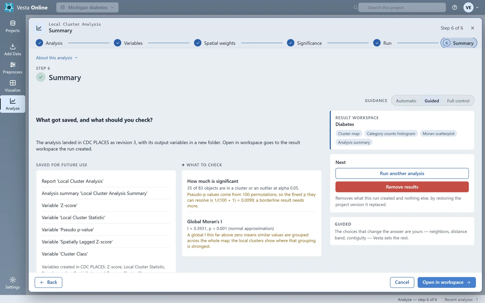
The run adds five variables to the CDC PLACES dataset: a standardized value, the local cluster statistic, its pseudo-p value, the cluster class and the spatially lagged standardized value.
The result
Section titled “The result”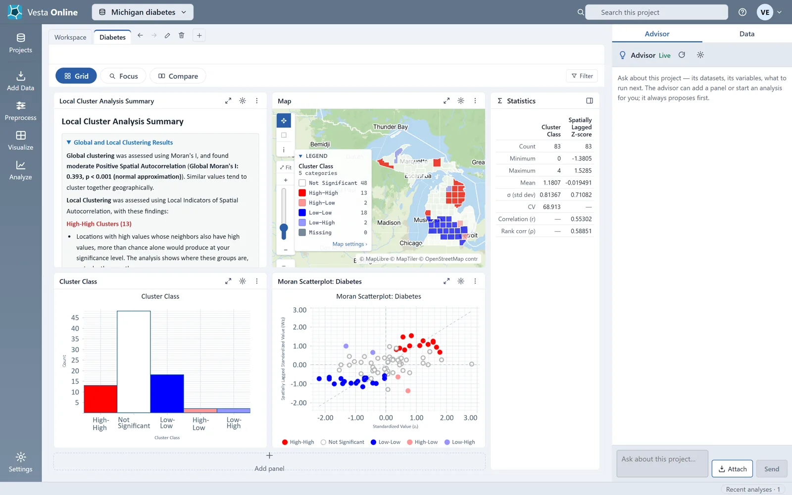
Each county is classed as High-High, Low-Low, High-Low, Low-High or Not Significant. High-High and Low-Low are clusters; High-Low and Low-High are outliers, values unlike their surroundings.
Where next
Section titled “Where next”- Bring in your own file or another source: Importing data.
- What the cluster classes mean and how to tune the analysis: Local cluster analysis.
- Model what drives the pattern: Regression and GWR.
- Estimate values between sample points: Kriging.
- Share the project with a colleague: Sharing.
Not sure which method fits your question? When the Advisor is turned on, you can describe your question on the Analysis step and let the Advisor suggest one. The Advisor is an optional AI-assisted guided workflow; see Using the Advisor.