Scan statistics
Find clusters of cases in space, or in space and time, with the spatial and space-time scan statistics in Vesta Online.
A scan statistic looks for clusters of cases: places, or places and times, where the case rate is higher (or lower) than the rest of the data would predict. It moves a window across the study area, scores every window, and reports the ones that stand out most. This article runs the space-time scan on the highly pathogenic avian influenza outbreaks in the Avian influenza in Europe sample: 3,443 outbreak records, 3,375 of which fall on the grid, counted by month onto a 50 km grid, October 2021 to September 2023. The space-time scan uses a cylinder: a circle in space over a run of consecutive months. Every step below was run on Vesta Online, and the screenshots come from that run. The spatial scan, which has no time dimension, is described after the steps.
The six steps
Section titled “The six steps”- Open a project that holds your dataOpen the Projects page, select a project and choose Open Project. This walk-through uses a copy of the Avian influenza in Europe sample, whose 50 km grid dataset has 1,664 cells and 24 monthly time periods, with the outbreaks counted onto each cell (HPAI outbreaks - Count) and the chickens it holds, as the population (HPAI outbreaks - Exposure).
- Choose Space-time scan statisticChoose Analyze in the left rail, then Find clusters & hotspots, then choose Space-time scan statistic. The analysis has five steps: Analysis, Variables, Cluster size, Run and Summary.
- Pick the cases and the populationOn Variables choose the dataset, 50 km grid. Leave the Scan model on Poisson, which divides a case count by a population, and pick HPAI outbreaks - Count as the Case variable and HPAI outbreaks - Exposure as the Population variable. Leave the Scan direction on High rates, which reports clusters of excess only. The side card shows the 1,664 locations and the 24 time periods scanned. Choose Next: Cluster size.
- Set the cluster sizeSwitch Guidance to Full control, so the replications and the seed are on the screen. Set Maximum spatial size to 0.10, so no window holds more than 10% of the total population. Set Maximum temporal size to 0.20, so no cylinder is taller than 20% of the study period, about five of the 24 months. Leave Maximum secondary clusters at 10, Monte Carlo replications at 999 and Seed at 42. Choose Run analysis.
- Run the analysisThe run happens on the server. Stay on the step: it reports there until it finishes, which took about three minutes here. If you start a second run while another of yours is going, the step says Another analysis of yours is still running. The Summary then lists what was saved and what to check.
- Open the result workspaceChoose Open in workspace. The result workspace has the Space-Time Scan Summary, a map of the clusters, the Space-Time Scan Cluster Summary table, the Space-Time Scan Diagnostics table and a statistics panel. It opens on the time step inside the most likely cluster's period, April 2022 here, and the map legend lists the clusters with the number of cells each has in that month; use the time slider to move to another month.
What you should see
Section titled “What you should see”The method
Section titled “The method”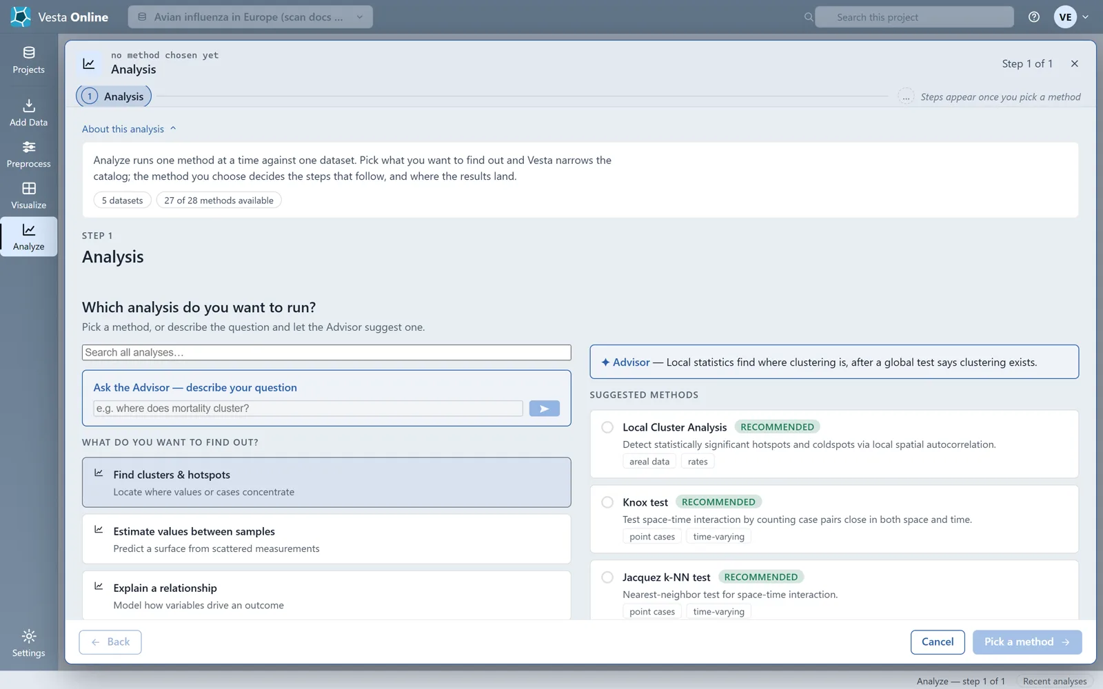
The cases and the population
Section titled “The cases and the population”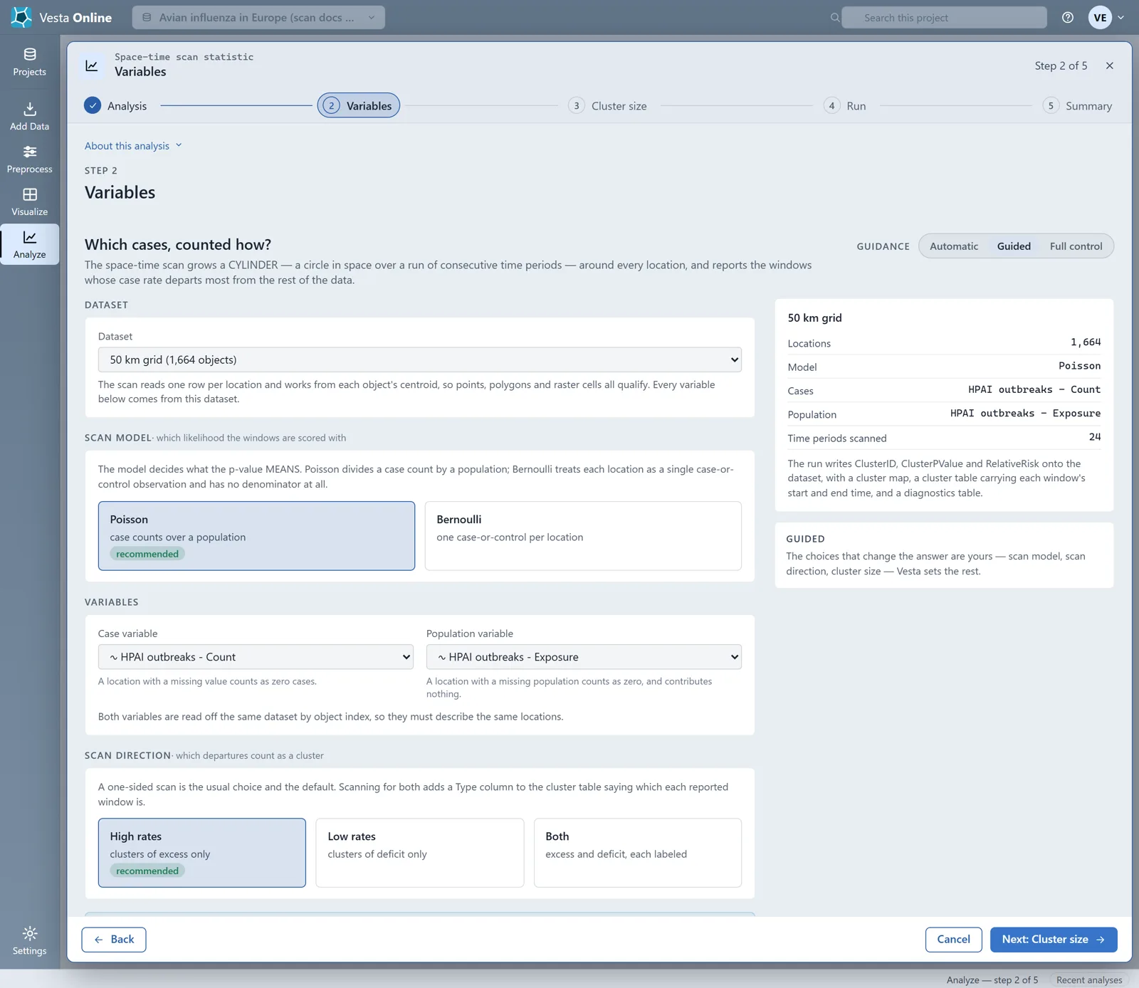
The scan reads one row per location and works from each object’s centroid, so points, polygons and raster cells all qualify. Both variables come from the same dataset and are matched by object index, so they must describe the same locations. A location with a missing value counts as zero cases, and a location with a missing population counts as zero and contributes nothing.
The Scan model decides what the p-value means. Poisson divides a case count by a population. Bernoulli treats each location as a single case-or-control observation and has no denominator at all, so it asks for no population variable. The space-time scan offers no Multinomial model; only the spatial scan does.
If the dataset carries only one time period, the step warns that the space-time scan has nothing to add: with a single period the cylinder has no height and the run reduces to a spatial scan, so use the spatial scan instead.
The cluster size
Section titled “The cluster size”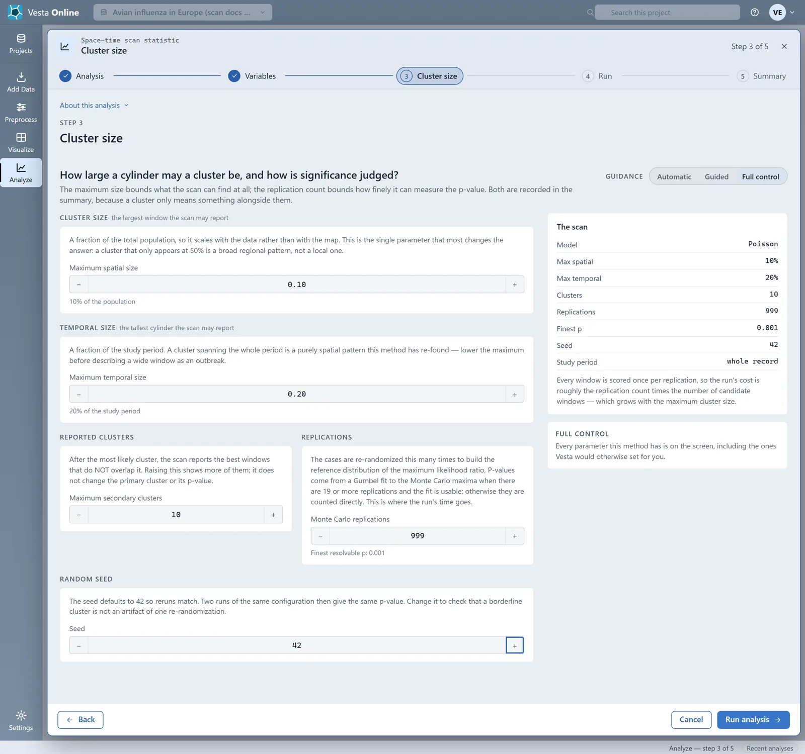
Each setting is a limit on what the scan may report:
- Maximum spatial size The largest window, as a fraction of the total population (0.01 to 1.00, default 0.50). It scales with the data, not with the map, and it changes the answer more than any other setting: a cluster that only appears at 50% is a broad regional pattern, not a local one.
- Maximum temporal size The tallest cylinder, as a fraction of the study period (0.01 to 1.00, default 0.50). A cluster spanning the whole period is a purely spatial pattern this method has re-found, so lower the maximum before describing a wide window as an outbreak.
- Maximum secondary clusters After the most likely cluster, the scan reports the best windows that do not overlap it (1 to 100, default 10). Raising it shows more of them; it does not change the primary cluster or its p-value.
- Monte Carlo replications How many times the cases are re-randomized to build the reference distribution (1 to 100,000, default 999). The step shows the finest p-value that many replications can resolve, 1 divided by the replications plus one, which is 0.001 for 999. Below about 99 replications the step warns that the p-values are too coarse.
- Seed The starting point of the re-randomization (default 42). The same configuration and seed give the same p-values; change it to check that a borderline cluster is not an artifact of one re-randomization.
At the default Guided level only the two sizes are yours; Vesta sets 10 clusters, 999 replications and the seed 42. Every window is scored once per replication, so the run’s cost is roughly the replications times the number of candidate windows, which grows with the maximum size. The step has no study-period control: the side card lists the Study period as whole record, and the scan covers every period in the dataset.
The summary
Section titled “The summary”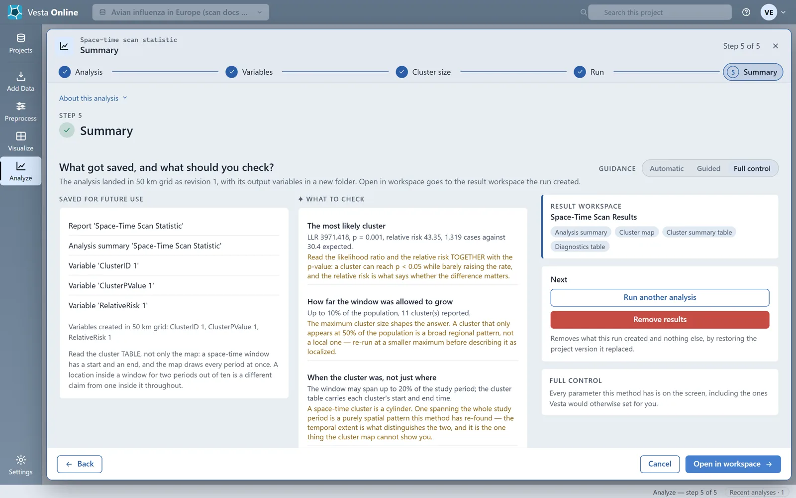
The run adds three variables to the 50 km grid dataset: ClusterID, ClusterPValue and RelativeRisk. Under What to check the Summary reports the most likely cluster, here a log-likelihood ratio of 3971.418, p = 0.001, a relative risk of 43.35 and 1,319 cases against 30.4 expected. It repeats the limits you set, 10% of the population and 20% of the study period, and the 11 clusters reported. Read the likelihood ratio and the relative risk together with the p-value: a cluster can reach p below 0.05 while barely raising the rate.
Reading the result
Section titled “Reading the result”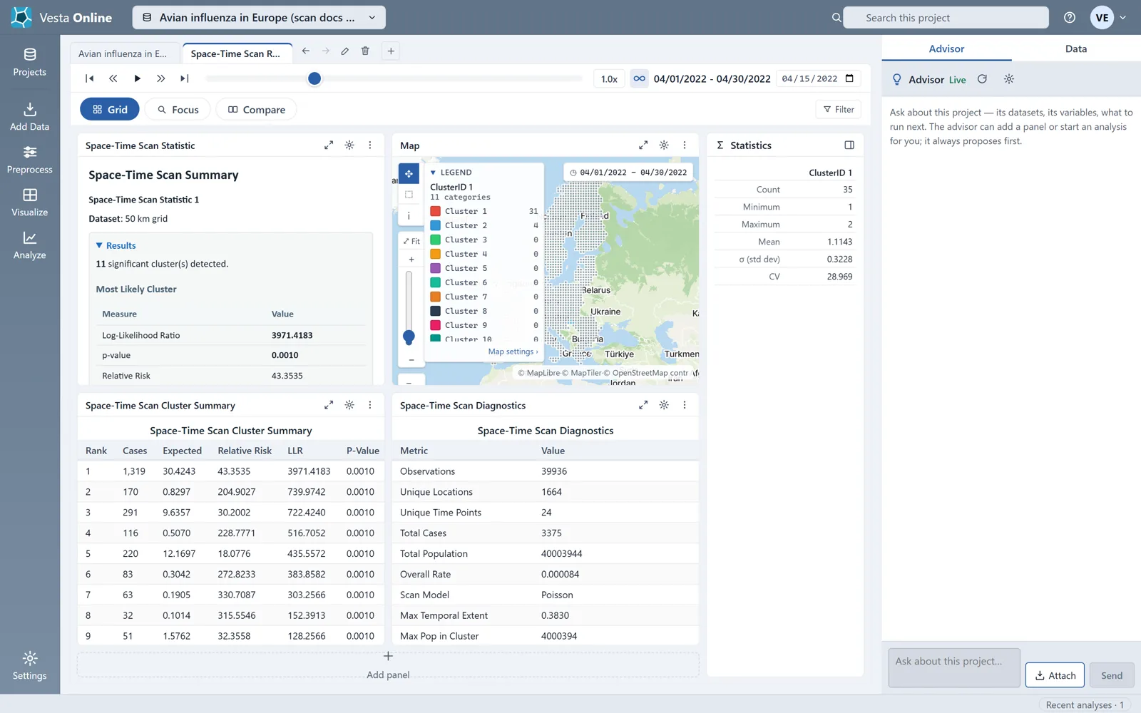
The Space-Time Scan Summary opens with the number of significant clusters, then the most likely cluster: its log-likelihood ratio, p-value, relative risk and the observed and expected cases, and the scan configuration. The map colors each cell by ClusterID, one entry for each of the 11 clusters and one for Not in cluster, and the legend counts the cells in each for the month on the time slider. In April 2022 that is 31 cells in Cluster 1, 4 in Cluster 2 and none in the others, because the other clusters occur in other months.
The scan reported 11 clusters, every one at p = 0.001. The first five, from the Space-Time Scan Cluster Summary:
| Rank | Cases | Expected | Relative risk | Start to end |
|---|---|---|---|---|
| 1 | 1,319 | 30.42 | 43.35 | February to June 2022 |
| 2 | 170 | 0.83 | 204.90 | April to May 2022 |
| 3 | 291 | 9.64 | 30.20 | November to December 2021 |
| 4 | 116 | 0.51 | 228.78 | November 2022 to March 2023 |
| 5 | 220 | 12.17 | 18.08 | January to February 2023 |
The most likely cluster is 1,319 outbreaks over five months, against about 30 expected. Rank 2 is smaller and shorter but far more intense, a relative risk of 205. Relative risk compares the rate inside the window with the rate outside, so a value of 43 means about 43 times the rate. The table also lists ranks 6 to 11, which have 32 to 83 cases each.
Read the cluster table, not only the map: a space-time window has a start and an end, and the map draws every period at once. A location inside a window for two months out of five is a different claim from one inside it throughout.
Every p-value in the cluster table is 0.0010. The Cluster size step says how the p-values are reached: from a Gumbel fit to the Monte Carlo maxima when there are 19 or more replications and the fit is usable, otherwise counted directly. The Space-Time Scan Diagnostics table lists the p-value method as Gumbel Approximation, which is that fit, with its two parameters, beside the replications, the number of windows evaluated and the maximum likelihood ratio the replications reached (26.7, against 3971 observed). It also warns that 5,208 observations have zero population: cells with no chickens, which contribute nothing to the scan. A scan statistic says where and when cases cluster, not why; the cause needs covariates and context.
The spatial scan
Section titled “The spatial scan”The spatial scan has the same five steps and the same settings, without time. It grows a circular window around every location and reports the windows whose case rate departs most from the rest of the data, with a p-value for each. Maximum spatial size, Maximum secondary clusters, Monte Carlo replications and Seed work as above, and there is no Maximum temporal size. Its Scan model offers Multinomial as well as Poisson and Bernoulli: it takes two or more count columns, or one categorical column, as the categories, has no case variable, no population and no direction, and asks whether the mix inside a window differs from the mix outside it. The Summary offers an Analysis summary, a Cluster map, a Cluster summary table and a Monte Carlo histogram.
Where next
Section titled “Where next”- Another way to see where values cluster: Local cluster analysis.
- Not sure which method fits your question: Choosing a method.
- Bring in your own data: Importing data.
Not sure which method fits your question? When the Advisor is turned on, you can describe your question on the Analysis step and let the Advisor suggest one. The Advisor is an optional AI-assisted guided workflow; see Using the Advisor.