Joinpoint regression
Find the years a trend changes direction or steepness, and the average annual percent change, with Joinpoint regression in Vesta Online.
Joinpoint regression fits straight segments through a trend over time and finds the years where the direction or steepness changes. This article runs it on the Overdose death rate (per 100,000) for the 88 Ohio counties in the Ohio overdose trends sample, 2003 to 2021, as one statewide series. Every step below was run on Vesta Online, and the screenshots come from that run. For a shorter first run with the defaults, see the Quickstart.
The six steps
Section titled “The six steps”- Open a project that holds your dataOpen the Projects page, select a project and choose Open Project. This walk-through uses a copy of the Ohio overdose trends sample, whose Ohio counties dataset has 88 objects and 19 time periods.
- Choose Joinpoint regressionChoose Analyze, then Detect a trend over time, then Joinpoint regression, and choose Pick a method. The analysis has five steps: Analysis, Variables, Model, Run and Summary.
- Pick the variableOn Variables choose the dataset, Ohio counties, and the variable, Overdose death rate (per 100,000). It is one measure at a time, and a binary variable is not offered. An object with no valid observation at two distinct times is left out of the fit, not treated as zero. The side card shows the Most joinpoints the timeline supports; here it is 3, so the run fits 4 candidate models: no joinpoint, then one per number of segments this timeline supports. It keeps the one with the lowest BIC. Choose Next: Model.
- Set the modelModel sets the scale, the series and the errors. Leave the scale on Log-Linear, the default, so the trend reads as an annual percent change. Under Group data by choose Combine all, one series over everything; the default, Separate by ID, fits one series per object. Under Errors choose Heteroscedastic and pick Death rate standard deviation, so a noisy year pulls the line less; the default, Homoscedastic, treats every observation as equally precise. The card on the right repeats what the run will fit. Choose Run analysis.
- Run the analysisThe run happens on the server. If you start a second run while another of yours is going, the step says Another analysis of yours is still running. The Summary then lists what was saved and what to check.
- Open the result workspaceChoose Open in workspace. The result workspace has the Joinpoint Regression Summary, a plot of the data and the fitted trend, two maps and a statistics panel.
What you should see
Section titled “What you should see”The method
Section titled “The method”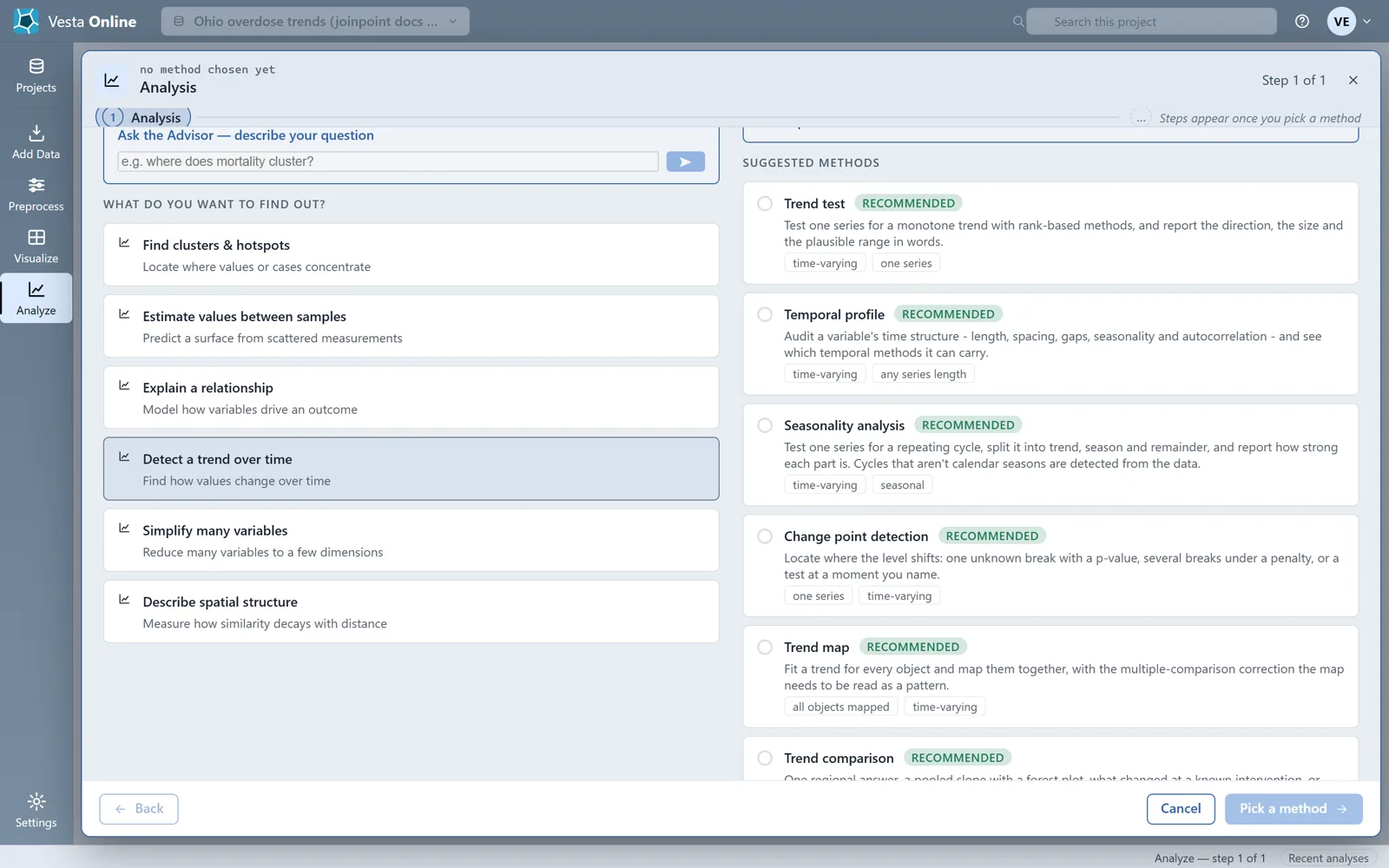
The variable
Section titled “The variable”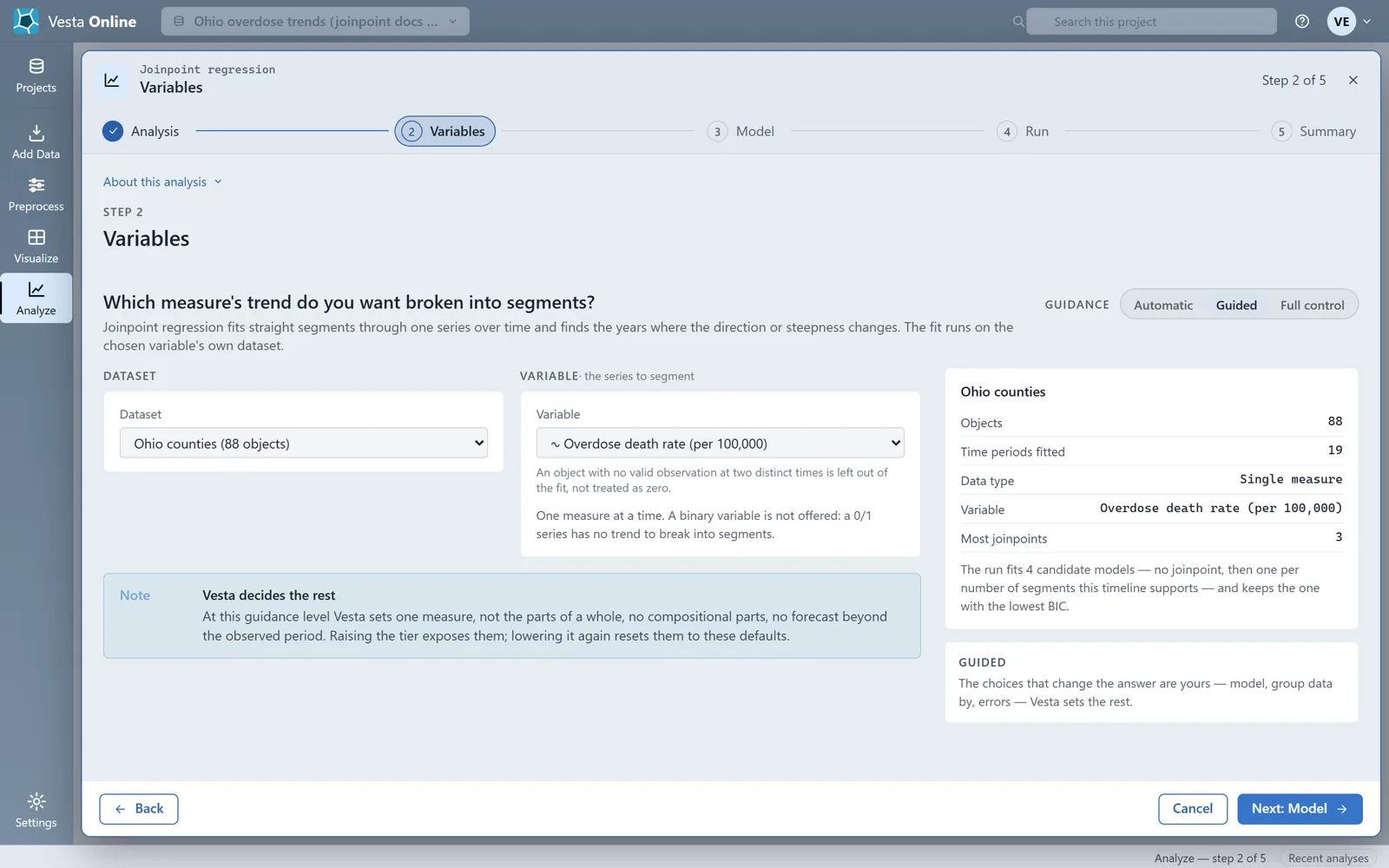
The model
Section titled “The model”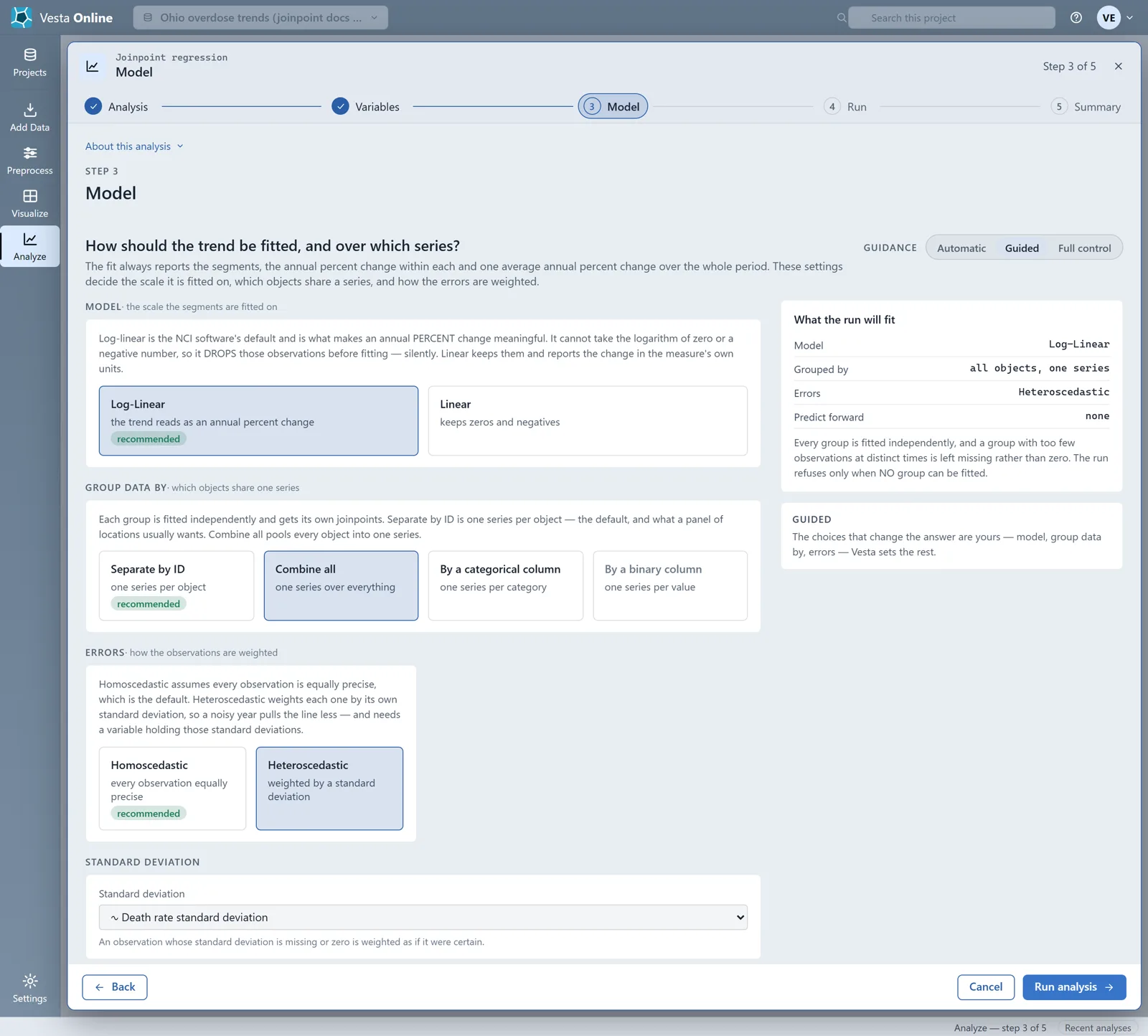
The summary
Section titled “The summary”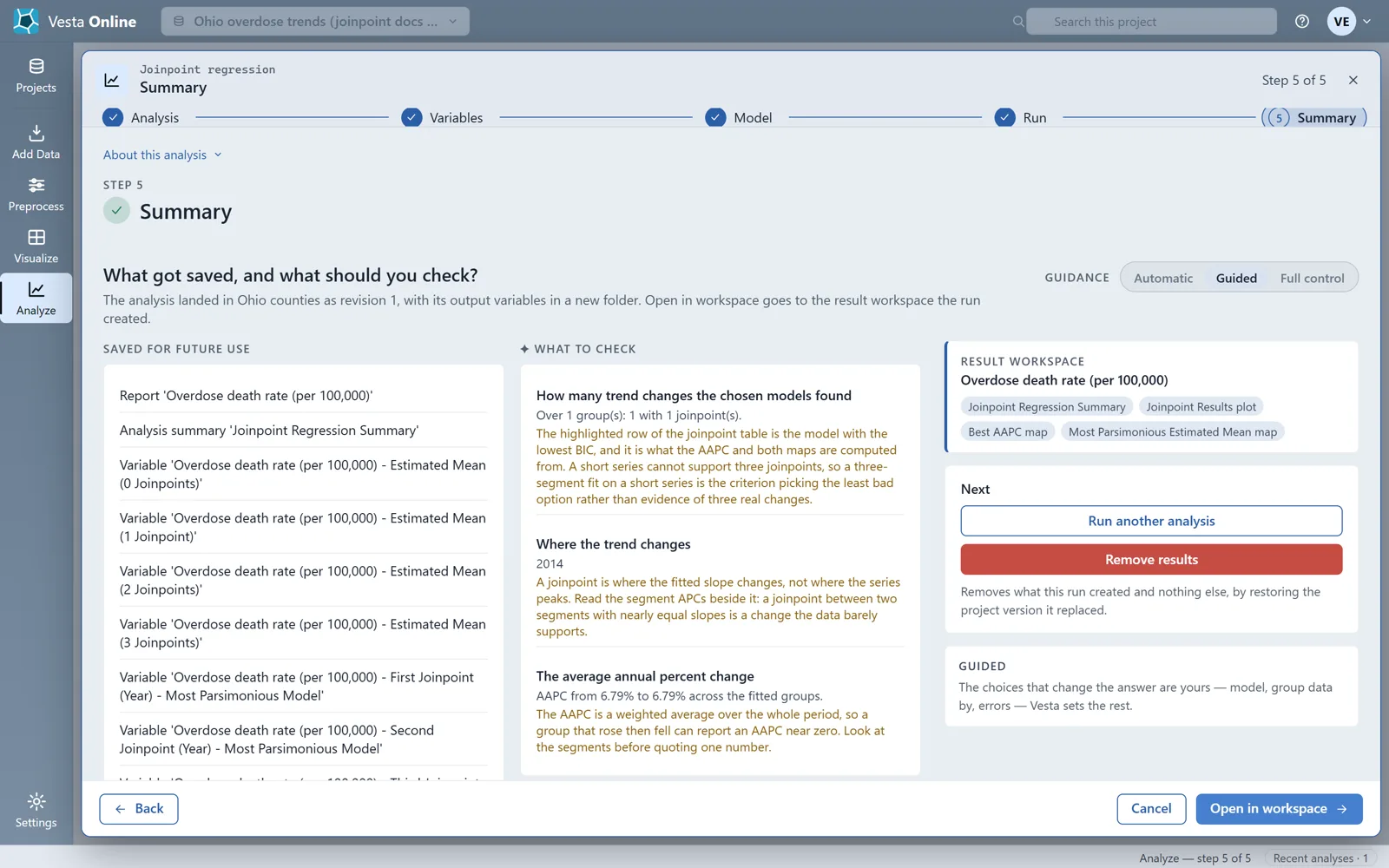
The run adds ten variables to the Ohio counties dataset: the estimated mean for each of 0, 1, 2 and 3 joinpoints, the years of the first, second and third joinpoint in the most parsimonious model, the most parsimonious model itself, its estimated mean and its AAPC. The Most Parsimonious Estimated Mean is what the chosen model fits at each location, and the Most Parsimonious AAPC is its average annual percent change: positive is rising, negative falling. A group with fewer joinpoints leaves the later joinpoint years missing, not zero.
The result
Section titled “The result”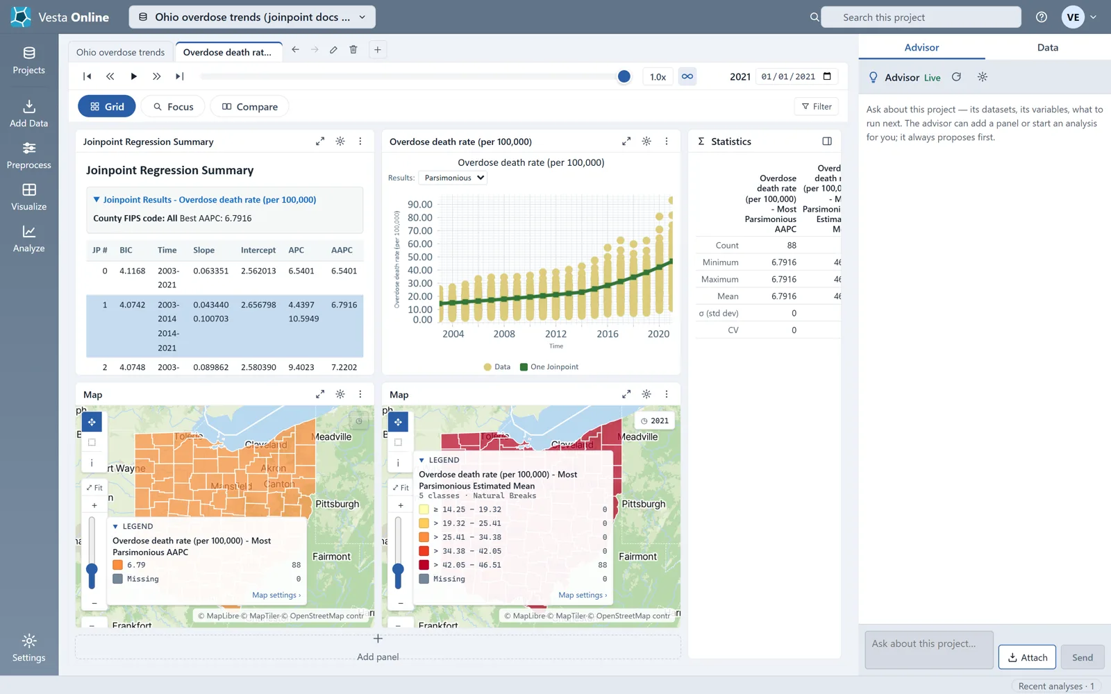
Reading the result
Section titled “Reading the result”The run fitted four models to the statewide series. The one with the lowest BIC is the most parsimonious, and the summary highlights its row:
| Joinpoints | BIC | Segments | APC (%) | AAPC (%) |
|---|---|---|---|---|
| 0 | 4.1168 | 2003 to 2021 | 6.54 | 6.54 |
| 1 (chosen) | 4.0742 | 2003 to 2014; 2014 to 2021 | 4.44; 10.59 | 6.79 |
| 2 | 4.0748 | 2003 to 2006; 2006 to 2013; 2013 to 2021 | 9.40; 2.83; 10.38 | 7.22 |
| 3 | 4.0807 | 2003 to 2006; 2006 to 2012; 2012 to 2018; 2018 to 2021 | 9.59; 2.57; 8.43; 13.72 | 7.48 |
The chosen model has one joinpoint, in 2014. The death rate rose about 4.4 percent a year from 2003 to 2014 and about 10.6 percent a year from 2014 to 2021, and the average annual percent change over the whole period is 6.79 percent. The BIC of the one-joinpoint model (4.0742) and the two-joinpoint model (4.0748) are very close, so the data barely separate them; read the segments beside the joinpoint rather than quoting one number. A joinpoint is where the fitted slope changes, not where the series peaks.
Because the run used Combine all, there is one group, so every county carries the same value in both result maps. The Best AAPC map is one orange, and its legend shows the one value, 6.79, for 88 counties, plus a Missing row at 0; a map of one value shows no pattern across the state.
Where next
Section titled “Where next”- Your first run, with the defaults: Quickstart.
- Another way to see where values cluster: Local cluster analysis.
- Bring in your own data: Importing data.
Not sure which method fits your question? When the Advisor is turned on, you can describe your question on the Analysis step and let the Advisor suggest one. The Advisor is an optional AI-assisted guided workflow; see Using the Advisor.