Co-kriging
Predict a variable using a second, correlated variable: fit a cross-variogram in Variography, save it, and krige through it in Vesta Online.
Co-kriging predicts one variable at places you did not measure, using a second variable that you measured at the same places and that is correlated with it. Vesta Online has no co-kriging method of its own: you build a model of both variables together in Variography, save it, and choose it in Kriging. This walk-through uses 840 soil samples from one field in southern Ontario. The variable is soil organic carbon (SOC, in percent), and the covariate is valley depth (VDepth), a terrain measure derived from elevation. Every step below was run on Vesta Online and the screenshots come from that run. For the single-variable path, see Kriging and Variography.
The data
Section titled “The data”The samples are from Laamrani, Voroney, Saurette, Berg, Blackburn, Gillespie and Martin (2022), Large dataset of soil organic carbon and topographic derivatives, Zenodo, https://doi.org/10.5281/zenodo.6611475, licensed CC BY 4.0. The published file has 840 rows and many terrain columns. This walk-through keeps six: the sample ID, SOC (%), Elev (elevation), VDepth and the coordinates X (DD) and Y (DD), which are WGS 84 degrees.
A covariate helps when it is correlated with the variable. In the 840 samples SOC has a correlation of 0.485 with VDepth, the strongest of the 54 topographic and NDVI columns of the published file (Pearson correlation over all 840 rows), and of -0.442 with Elev. This walk-through uses VDepth. The covariate has to be a numeric variable of the same dataset, measured at the same places as the variable.
The steps
Section titled “The steps”- Import the soil dataCreate a project and add the soil file from your PC (the Importing data article walks every screen). On the Geography step choose Build from coordinates and pick Y (DD) as the latitude and X (DD) as the longitude, then run the import. Vesta Online also reads the other columns as variables, so the dataset soc-covariates ends up with 840 objects and the variables SOC (%), Elev, VDepth, X (DD) and Y (DD).
- Choose VariographyChoose Analyze, then Describe spatial structure, then Variography, and choose Pick a method. The flow has seven steps: Analysis, Variable, Experimental, Model, Anisotropy, Save and Summary.
- Choose Full control and the variableOn Variable, set Guidance to Full control: the covariates card is only on this level. Choose the dataset soc-covariates and the variable SOC (%), and leave the value type on Continuous and the trend on None.
- Add the covariateTick Add covariates (cross-variogram for co-kriging), then pick VDepth from the Covariates list. It appears as a chip you can remove. Choose Next: Experimental.
- Read the cross-variogramThe plot is titled SOC (%) CoKriging Variogram. The Series list switches between the curve of SOC (%), the cross curve SOC (%) x VDepth and the curve of VDepth. The fit table lists an R-squared for each curve.
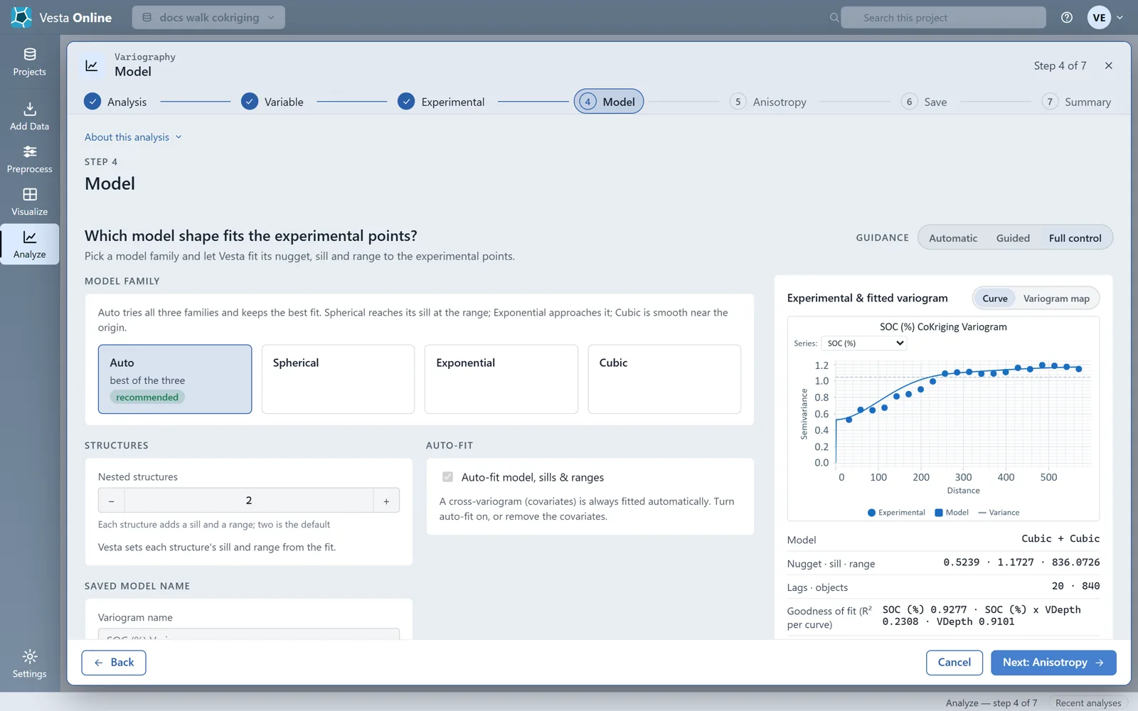
- Fit the modelOn Model, leave the family on Auto and the nested structures at 2. The auto-fit box is ticked and locked: a cross-variogram is always fitted automatically. Leave the name as it is, SOC (%) CoKriging Variogram, and choose Next: Anisotropy.
- Save the modelLeave anisotropy off and choose Save variogram. The Summary step lists the saved variogram model, a report and an analysis summary.
- Open the Variography resultChoose Open in workspace. The result workspace shows the model summary, the variogram plot with its series list, the variogram map and the fit card.
- Choose Kriging and the variableChoose Analyze, then Estimate values between samples, then Kriging. On Variables choose the dataset soc-covariates and the variable SOC (%), then choose Next: Variogram.
- Use the saved modelOn Variogram, choose Use a saved model and pick SOC (%) CoKriging Variogram from the Variogram model list. Choose Next: Prediction surface, leave the grid and neighbors at their defaults and choose Next: Options.
- Pick the kriging typeThe type list offers Ordinary, Simple and Standardized ordinary. Leave it on Ordinary. Choose Next: Validation, leave Cross-validation on None, and continue to Run.
- Run the krigingChoose Run analysis. The Summary step lists the report, the analysis summary, the grid and the two variables Kriging Estimate and Kriging Variance.
- Open the result workspaceChoose Open in workspace. The workspace holds the written summary, the estimate map, the variance map and statistics for both variables.
What you should see
Section titled “What you should see”The data
Section titled “The data”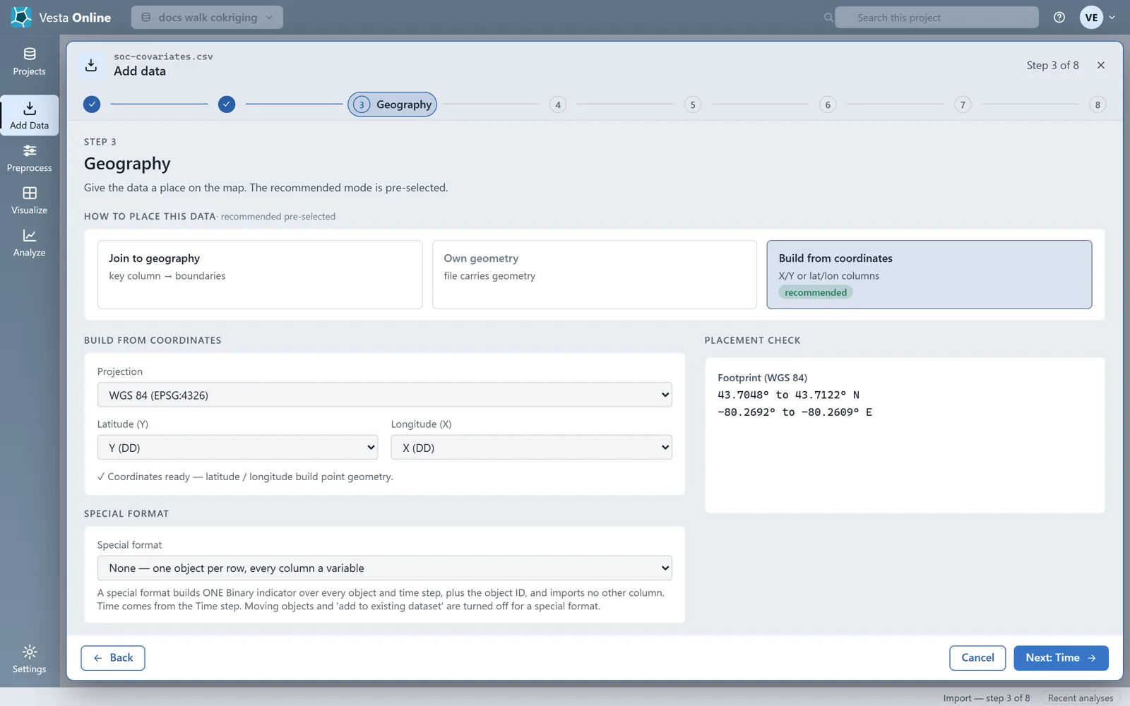
The covariate
Section titled “The covariate”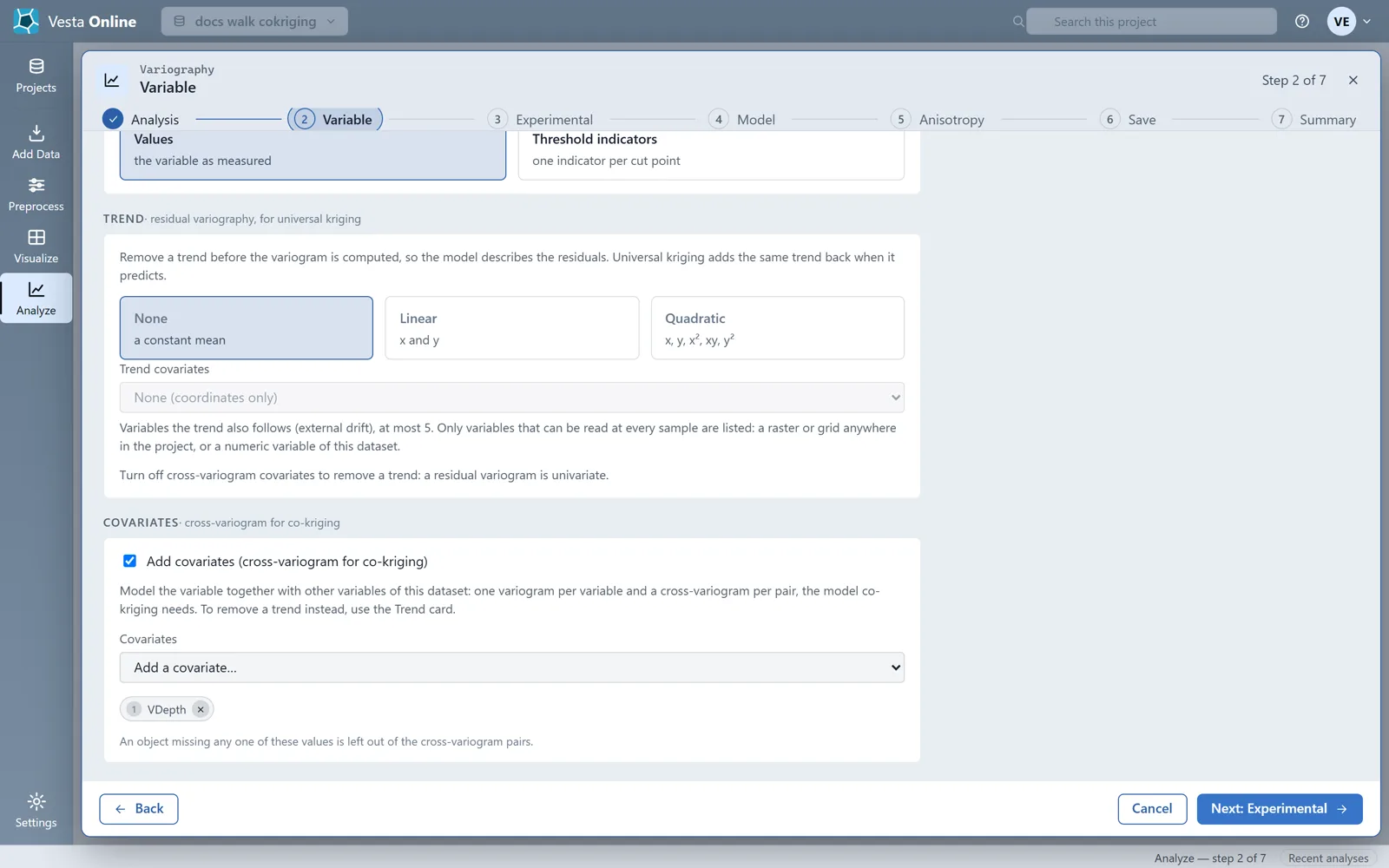
Co-kriging models the variable together with the covariates you add: one variogram per variable and a cross-variogram per pair, the model co-kriging needs. Up to 2 covariates can be added. An object missing any one of these values is left out of the cross-variogram pairs.
The covariates card is not available together with a trend: with covariates on, the Trend card says to turn off cross-variogram covariates to remove a trend, because a residual variogram is univariate. A compositional variogram is fitted without covariates too.
The cross-variogram
Section titled “The cross-variogram”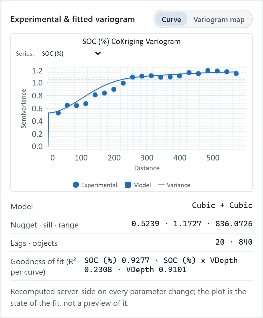
With one covariate the model has three curves: the variogram of SOC, the variogram of VDepth and the cross-variogram between them. All three share one set of structures and ranges, and Vesta fits them together, so there is no way to set the nugget, sill or range of one curve by hand: a cross-variogram (covariates) is always fitted automatically. In this run the model is two Cubic structures with a nugget of 0.5239, a sill of 1.1727 and a range of 836.07 m for SOC.
The R-squared for each curve says how well the model follows its points. The two single-variable curves fit closely (0.9277 for SOC and 0.9101 for VDepth) and the cross curve fits loosely (0.2308), so the covariate shares only part of its structure with SOC. A weak cross curve is a reason to check the covariate before you rely on the surface.
Saving and reading the Variography result
Section titled “Saving and reading the Variography result”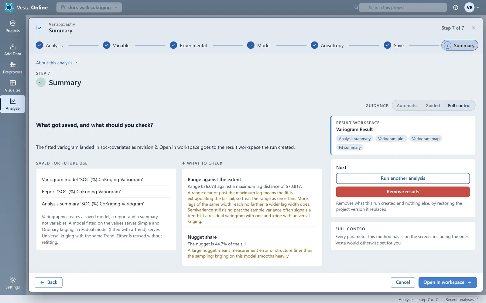
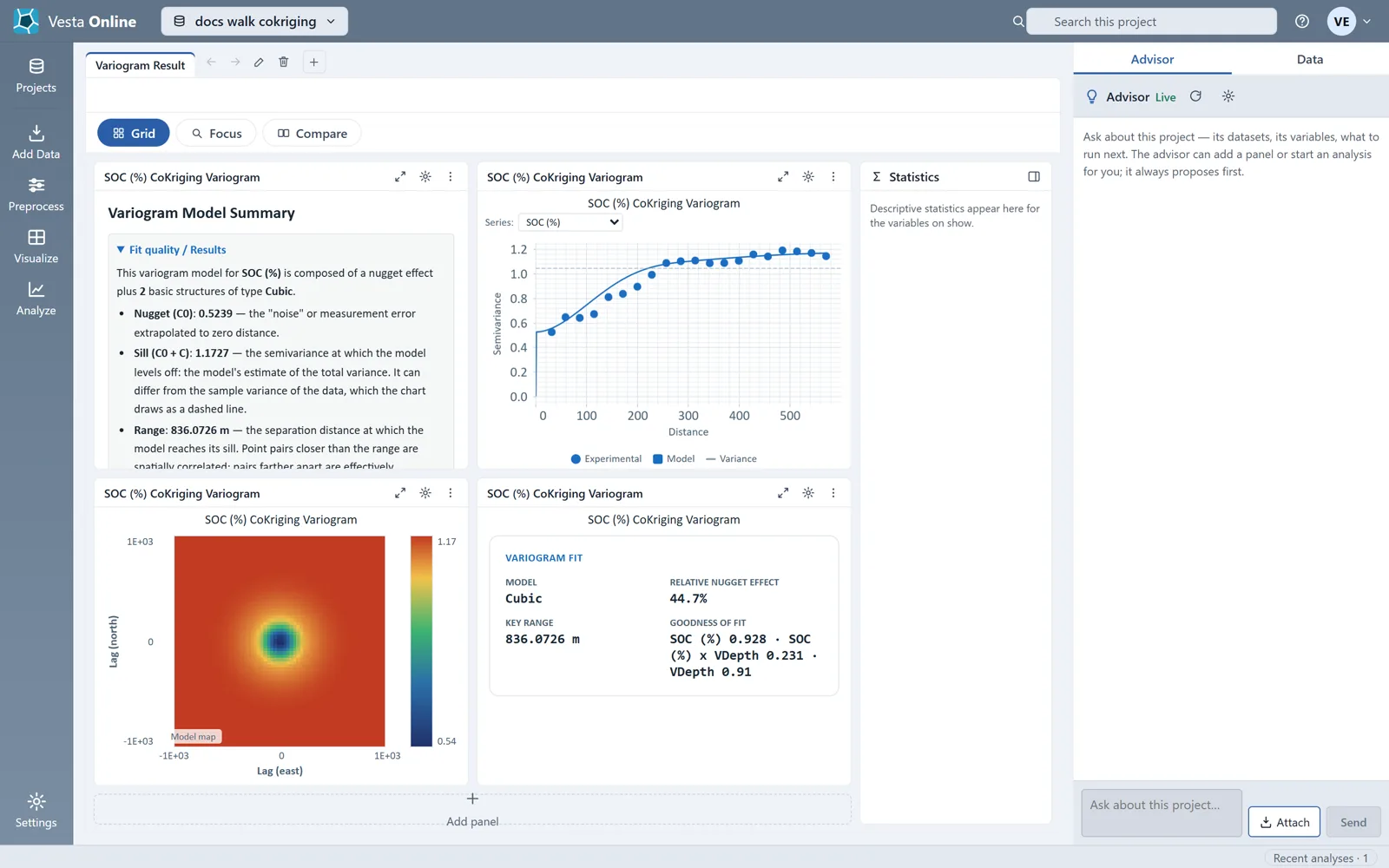
The Variography run saves a model, a report and a summary, not variables. The What to check card on the Summary step compares the range of 836.073 with a maximum lag distance of 570.817: the range is beyond the longest lag, so treat it as uncertain. The nugget is 44.7% of the sill, which the written summary calls moderate spatial dependence.
Kriging through the saved model
Section titled “Kriging through the saved model”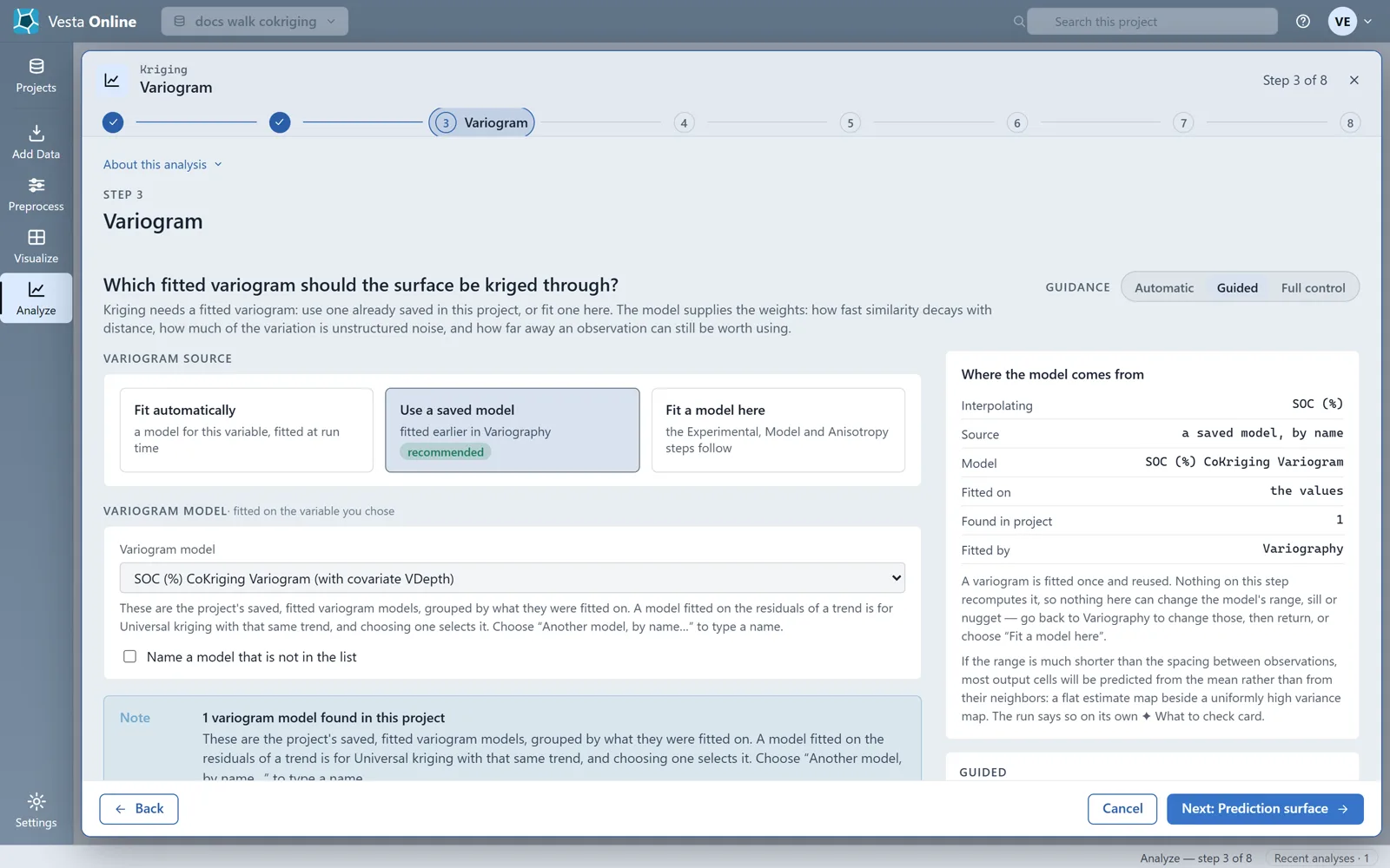
On the Variables step of Kriging, the page says the variogram model chosen on the next step must have been fitted on this same variable, and that Vesta stops the run otherwise rather than kriging one variable through another’s structure. This walk-through did not run the mismatch. To co-krige, you choose a cross-variogram fitted with covariates, and its covariates join the estimate. Kriging has no covariate control of its own: the covariates come from the saved model.
On the Variogram step, Use a saved model lists the project’s saved models by name; the default name of a covariate model says CoKriging. The side panel for this model reads Fitted on: the values.
In this run, Fit a model here after saving the covariate model gave a single-variable fit: its Experimental step was titled SOC (%) Variogram and showed one R-squared, 0.9793, and no Series list. To co-krige, use Use a saved model.
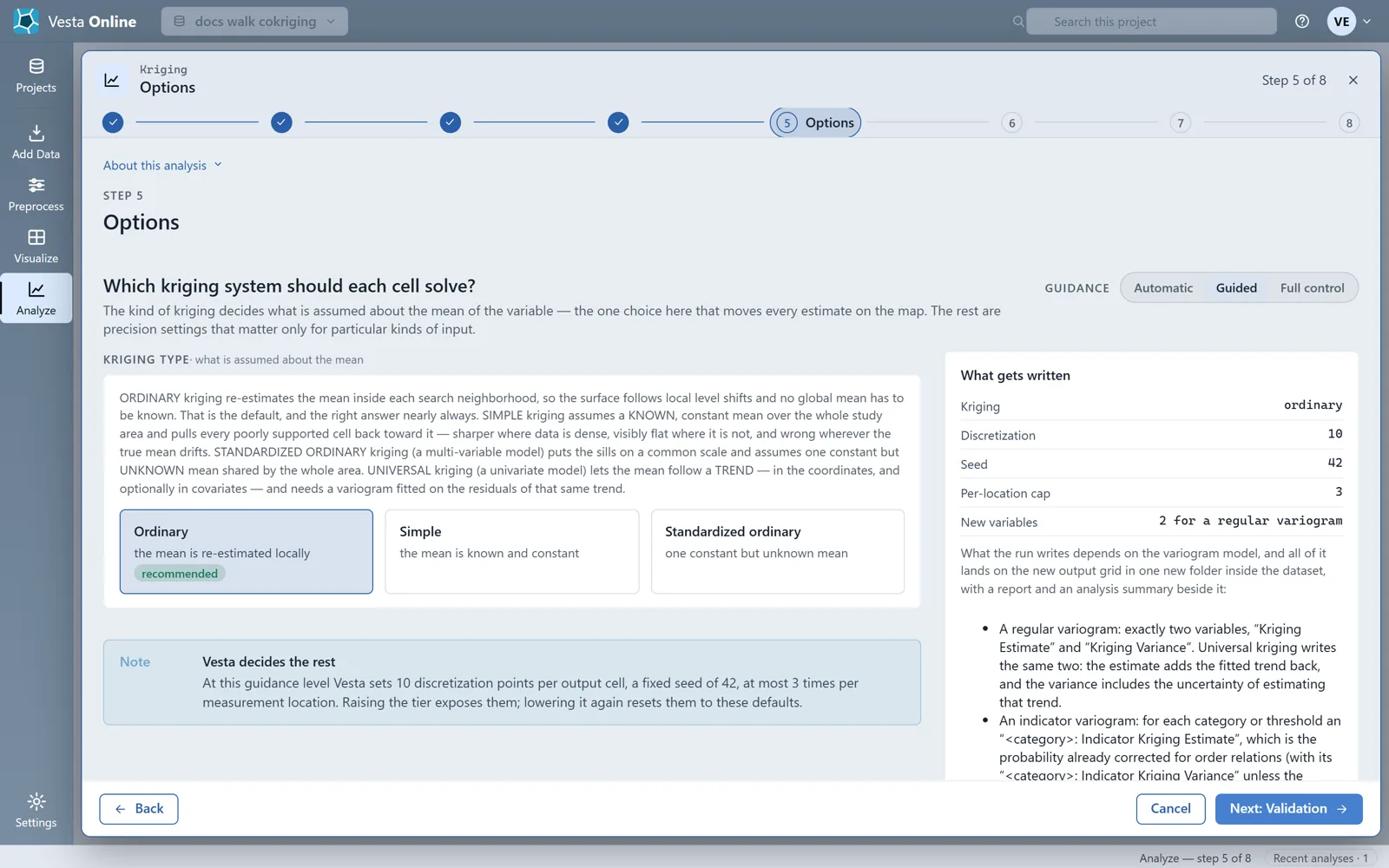
The kriging type list offers Ordinary, Simple and Standardized ordinary for this model. Universal kriging is univariate: a co-kriging (multi-variable) model cannot carry a drift. It is not offered. Standardized ordinary puts the sills on a common scale and assumes one constant but unknown mean for the whole area.
The result
Section titled “The result”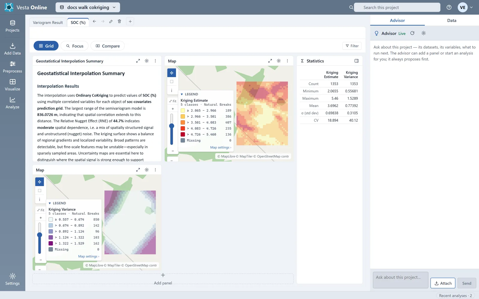
The Summary step of the run reads CoKriging: Cubic variogram, range = 836.073, over 1,353 output cells, and the written summary says the interpolation uses Ordinary CoKriging. The output is the same as single-variable kriging: a Kriging Estimate and a Kriging Variance variable on a new grid. In this run the estimate runs from 2.0655 to 5.46 with a mean of 3.6962, and the variance from 0.55681 to 1.5289.
As in any kriging, the variance depends on where the observations are, not on their values. This walk-through did not run kriging through a univariate model on the same data, so it does not show whether the covariate lowered the variance.
Limits
Section titled “Limits”Where next
Section titled “Where next”- Fit and save a variogram on its own: Variography.
- Run kriging with a model fitted automatically: Kriging.
- Bring in your own data: Importing data.