Importing data
Bring public data from the online catalog, or your own table, boundary file or GeoTIFF raster, into a Vesta Online project.
Vesta Online brings data into a project two ways: from its online catalog of public sources, or from a file on your computer. Both open from Add Data in the left rail, and both end on a Summary that says what landed. Every step below was run on Vesta Online; the screenshots come from that run. The four files used for the file steps are synthetic, made up for this page.
Import from the online catalog
Section titled “Import from the online catalog”The catalog is a curated set of public sources. This walk uses CDC PLACES, which Vesta Online offers at three geographic levels: County, Census Tract and ZCTA (ZIP Code Tabulation Area). All three import online.
- Pick a sourceOpen the project, choose Add Data in the left rail, and under From an online source choose the US Public Health category, then CDC PLACES. Choose Next: Geography.
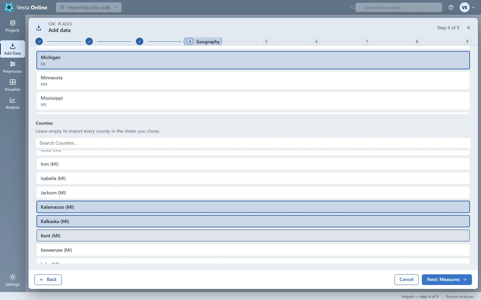
- Choose the geographyLeave Geographic level on County and pick a state under States. Counties then lists that state's counties; pick one or more, or leave it empty to import every county in the states you chose. The county choice narrows the import within the state: three counties picked give three records.
- Choose measures and release yearsChoose Next: Measures and pick Diabetes, then Next: Releases and pick 2023. Choose Next: Review. Review lists every choice, with an Edit button beside each, and a Dataset name you can change.
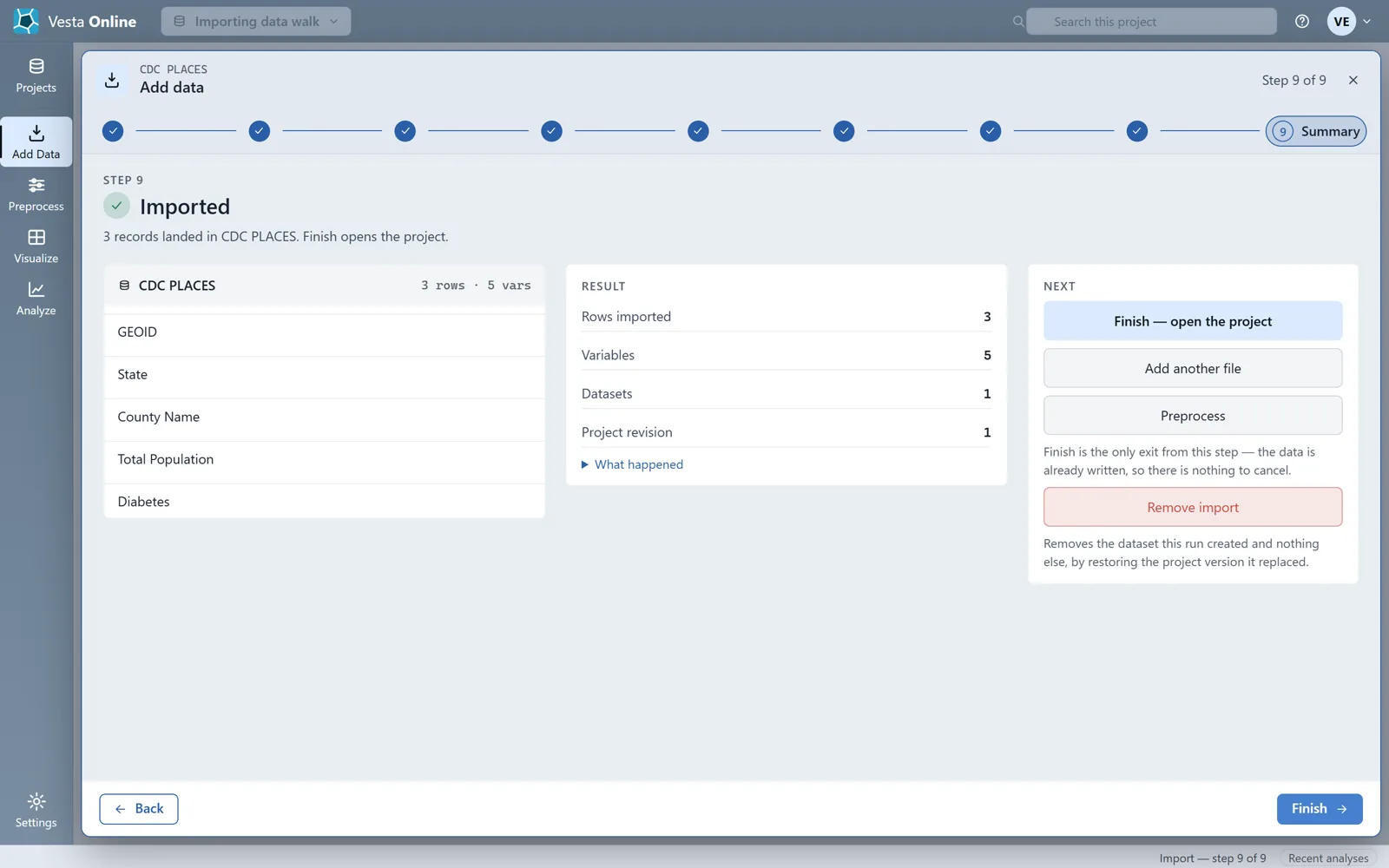
- Run the importChoose Run import. The fetch runs on the server, so stay on the page until the Summary appears. It reports the rows imported, the variables and the project revision.
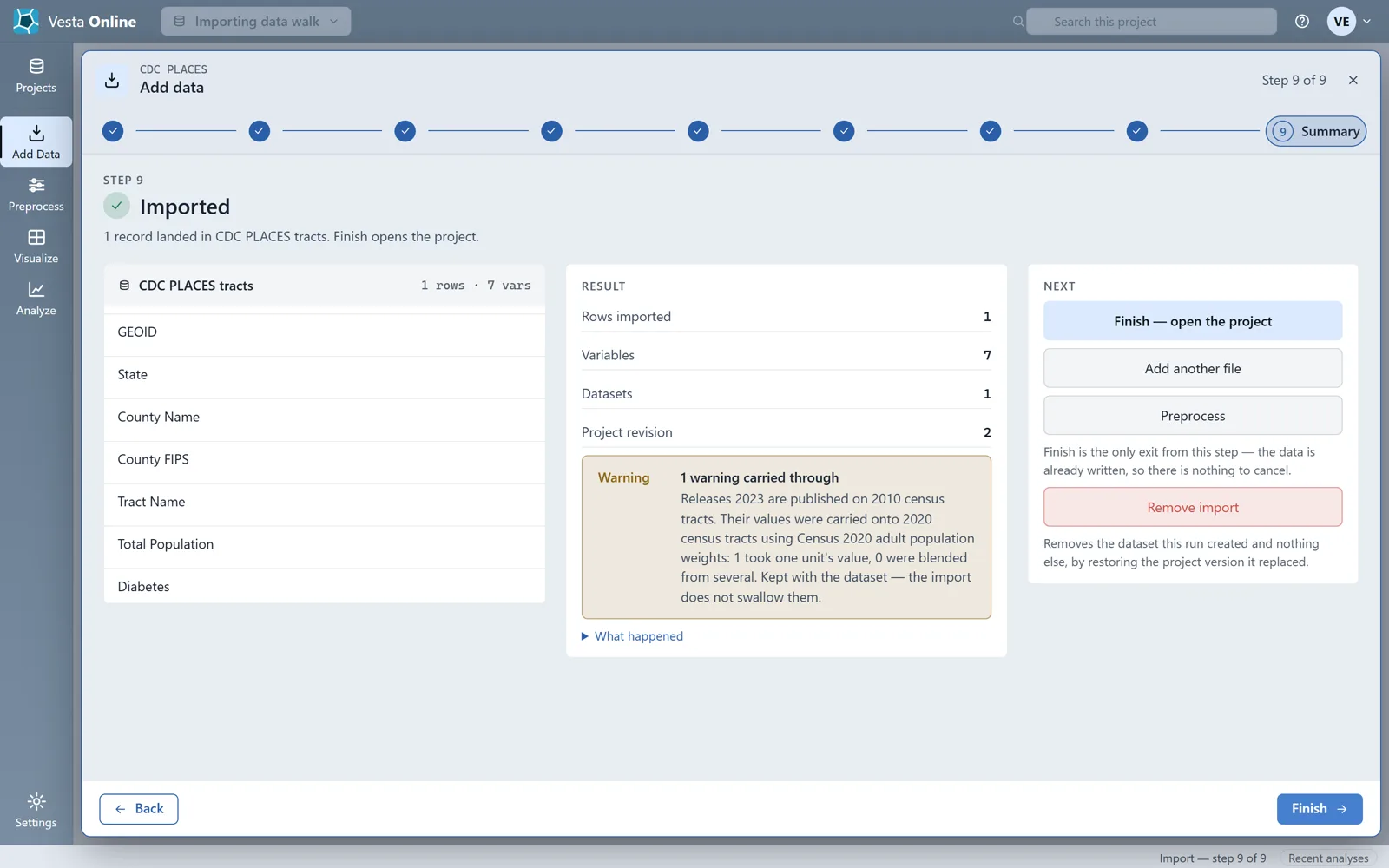
- Import census tractsRun the steps again, choosing Census Tract as the Geographic level, Michigan and one county. The state and county choices narrow a tract import the same way. This run imported the one tract of Keweenaw County.
The source and the geography
Section titled “The source and the geography”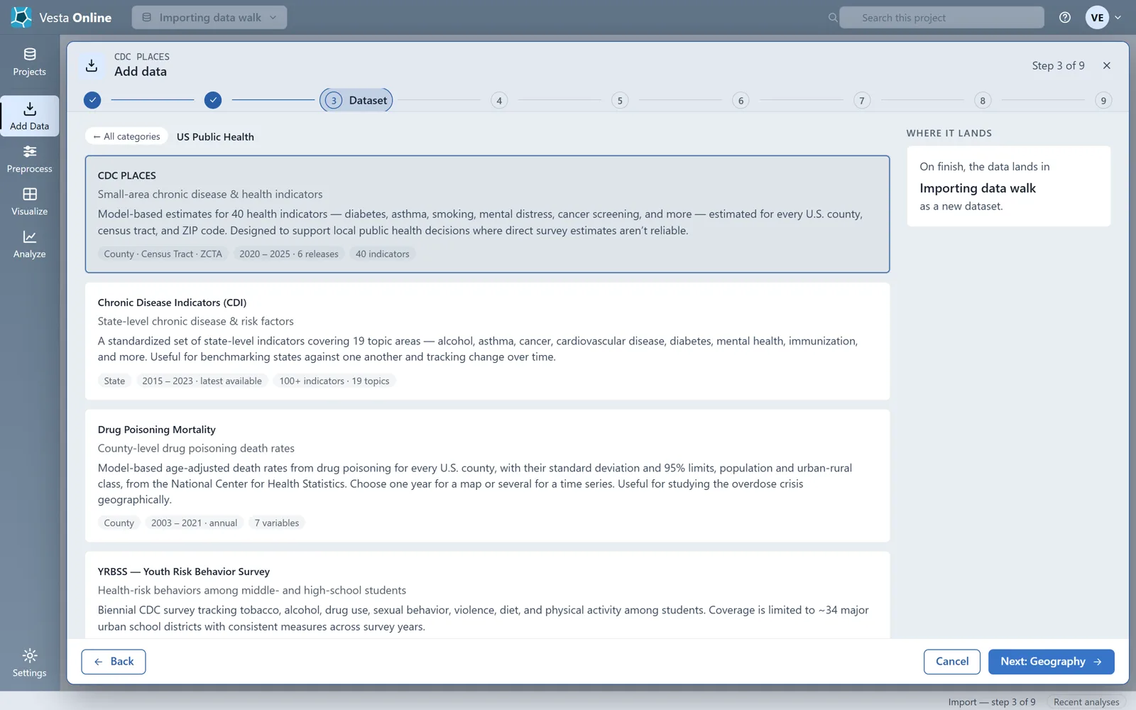
Review and Summary
Section titled “Review and Summary”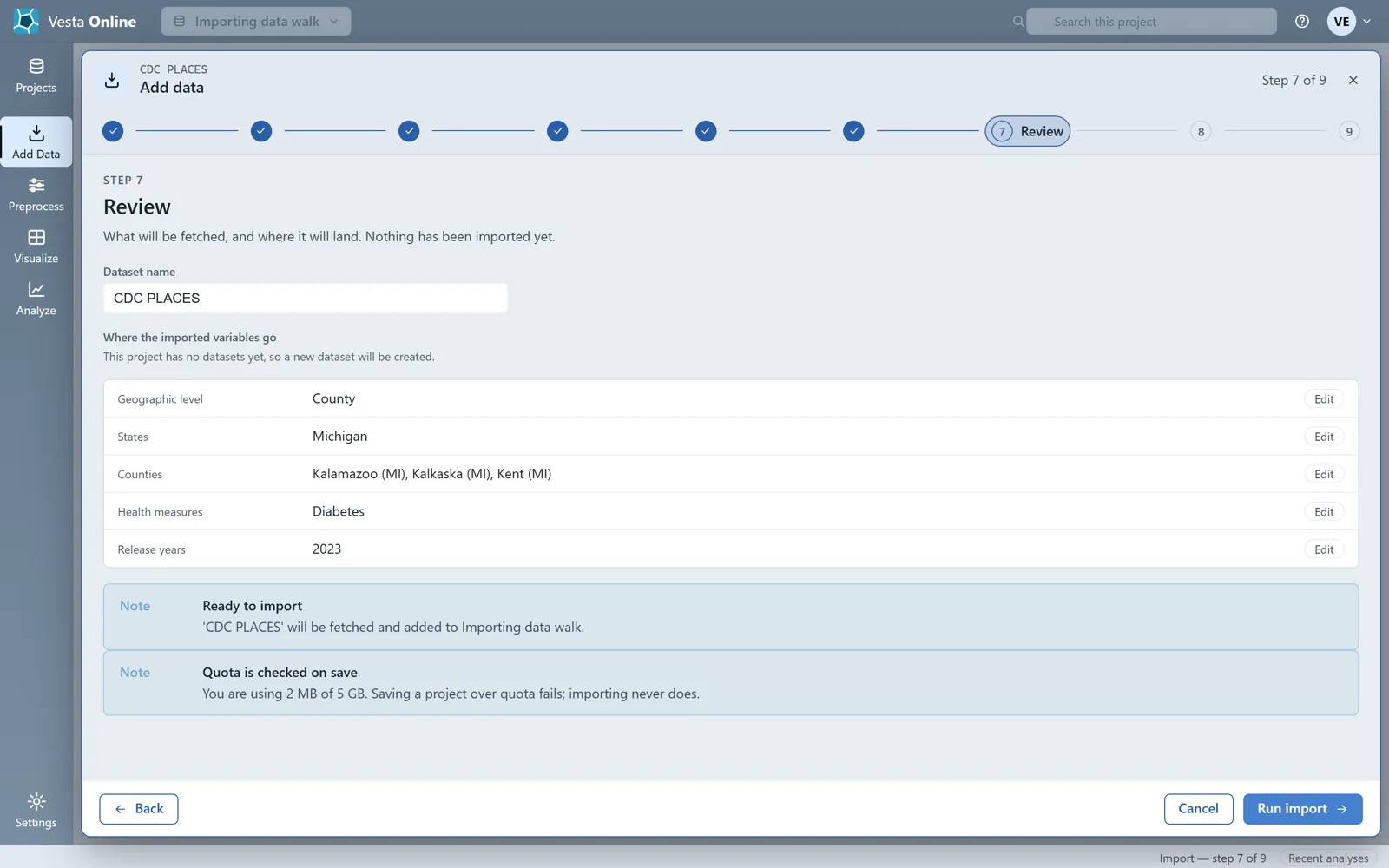
Boundary vintage
Section titled “Boundary vintage”Some PLACES releases are published on older, 2010 boundaries. When you import one, Vesta Online carries the values onto the 2020 boundaries and lists what it did as a warning on the Summary, as in the tract figure above. Read that warning before you map or analyze the dataset.
Import every ZIP Code Tabulation Area
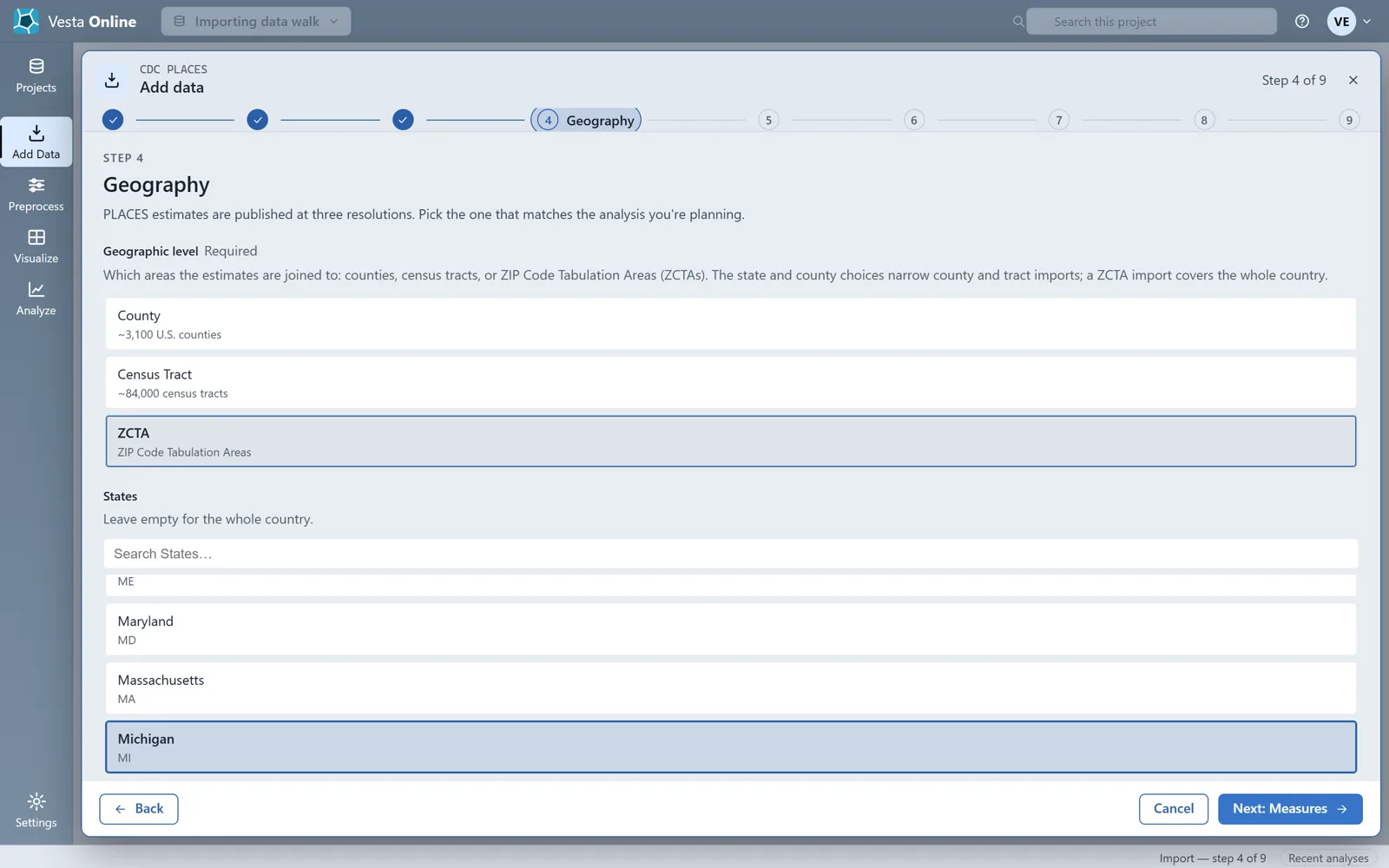
Section titled “Import every ZIP Code Tabulation Area”- Choose the ZCTA levelRun Pick a source again, then on Geography choose ZCTA as the Geographic level. A ZCTA import covers the whole country and ignores the States and Counties choices: the Review step does not list the state.
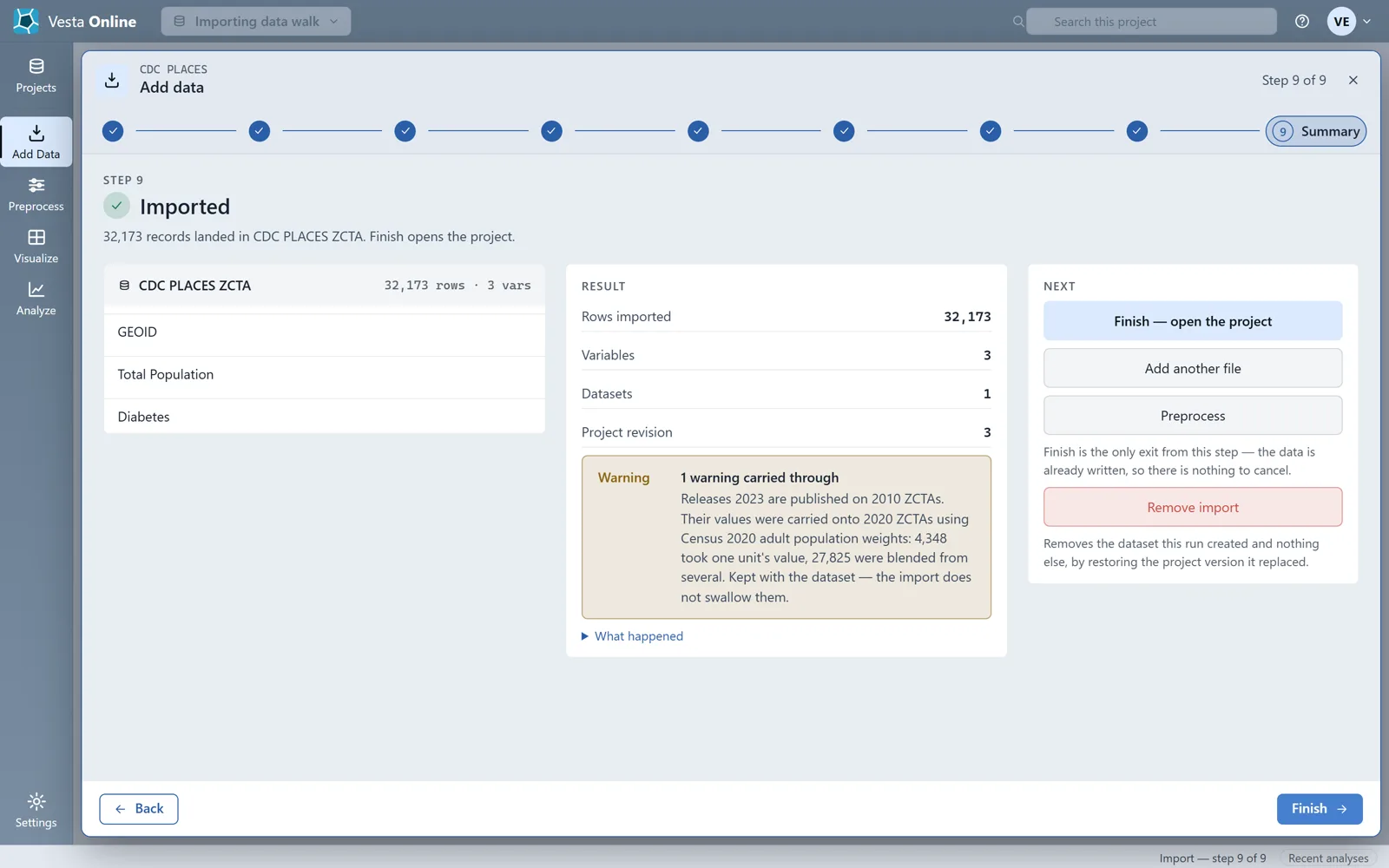
- Run the ZCTA importChoose Next: Measures, Next: Releases and Next: Review. Because this project already holds a dataset named CDC PLACES, rename the new one on Review (here, CDC PLACES ZCTA) so you can tell them apart, then choose Run import. This run imported 32,173 records and 3 variables.
Import a file
Section titled “Import a file”The file import has eight steps, and Next stays disabled until the current step has what it needs. This walk imports a small synthetic CSV of 20 made-up sites with latitude and longitude columns, joins a second synthetic CSV to county boundaries, and imports a small synthetic GeoTIFF.
- Choose a fileChoose Add Data in the left rail, then From a file on this PC. Drop a file on the page or browse for it. Vesta Online uploads it and reports what it detected: here a delimited table, CSV, 20 rows by 7 columns, comma delimiter, header in row 1, and a suggestion to build from coordinates. Choose Confirm & continue.
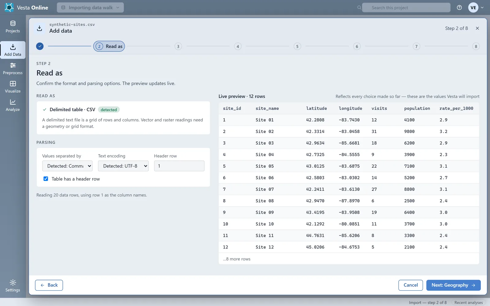
- Confirm how the file is readRead as shows the separator, the text encoding and whether the table has a header row, with a live preview of the values Vesta will import. Change any of them and the preview updates. Choose Next: Geography.
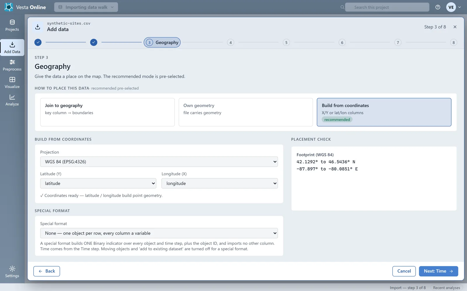
- Place the data on the mapGeography offers three ways to place the data: Join to geography, Own geometry and Build from coordinates. For this file Build from coordinates is pre-selected with latitude and longitude already chosen, WGS 84 as the projection and a footprint check. Choose Next: Time.
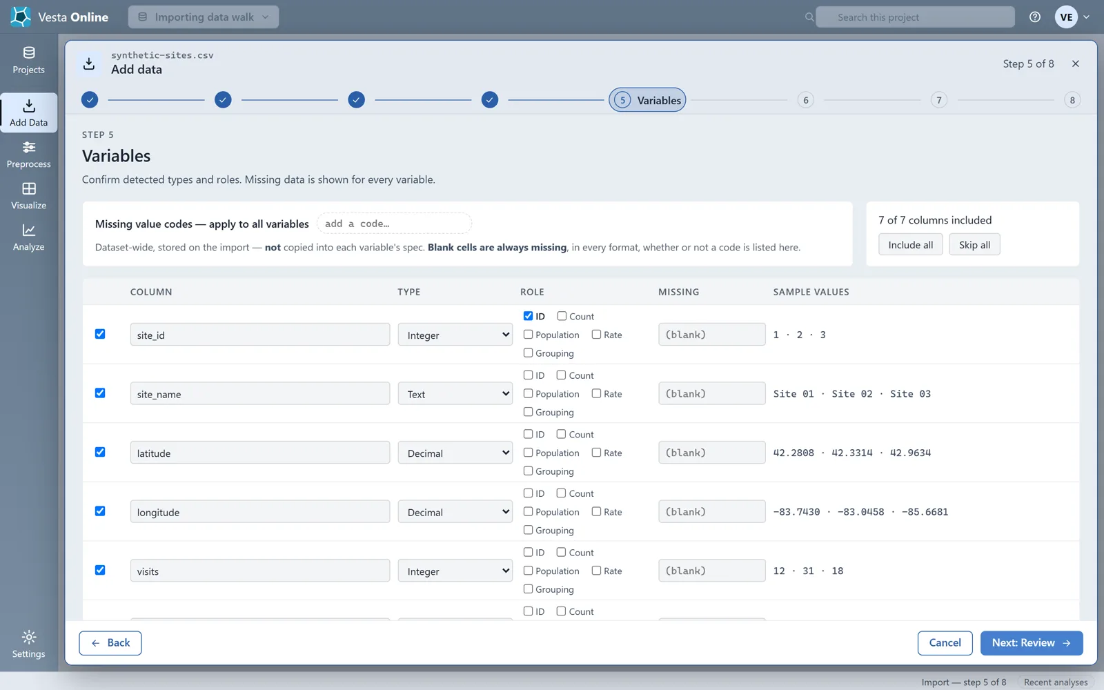
- Set time and check the variablesTime offers Field-derived, Set manually or Always valid; this file has no time column, so it stays on Always valid. Choose Next: Variables. Variables lists every column with its type, a role (ID, Count, Population, Rate or Grouping) and a missing-value code box. Choose Next: Review.
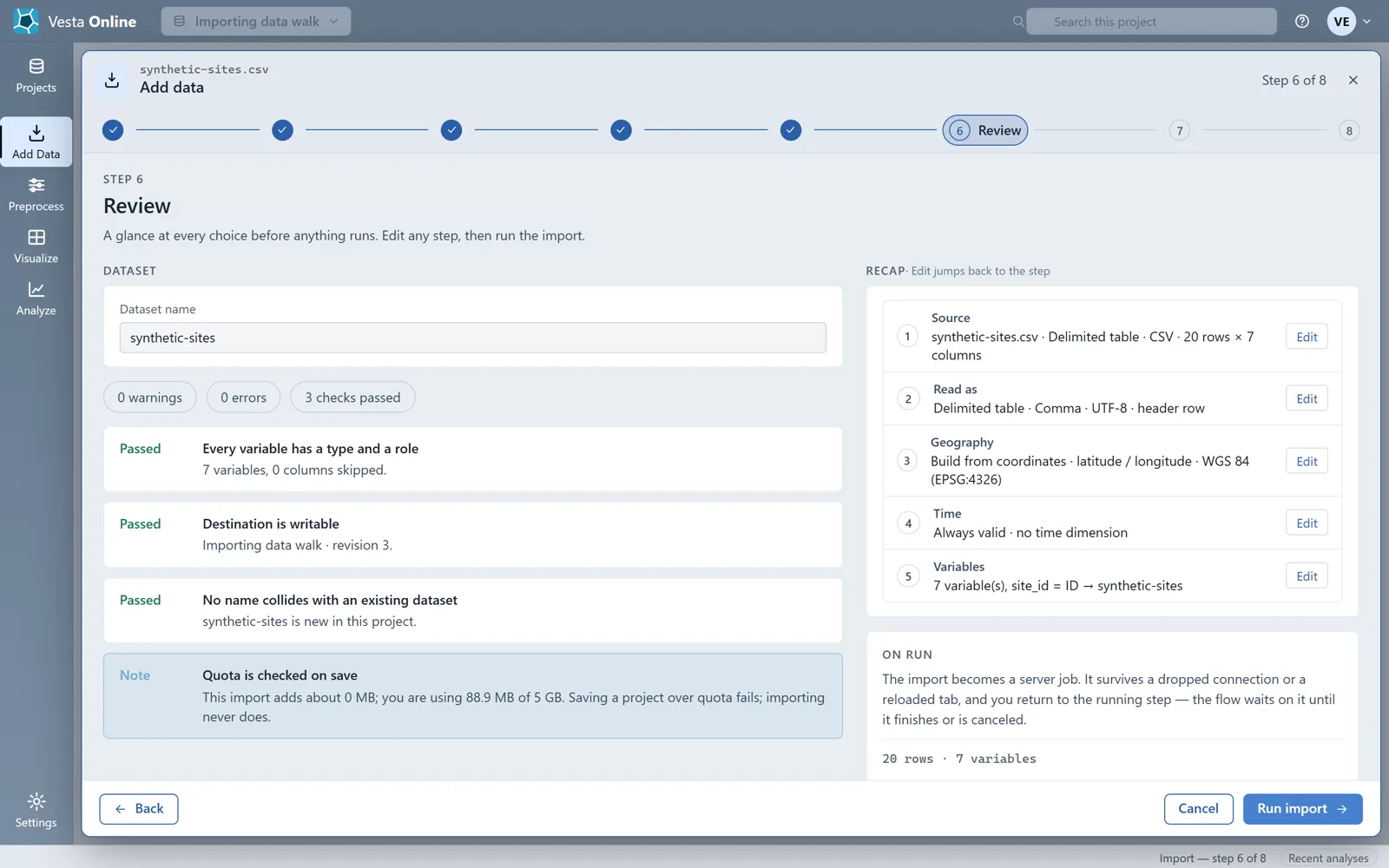
- Review the choicesReview gives the dataset a name and shows a recap of every step, each with an Edit button that jumps back to it, plus checks that passed. Choose Run import.
- Run the file importThe import runs as a server job. When it finishes the Summary reports 20 rows and 7 variables.
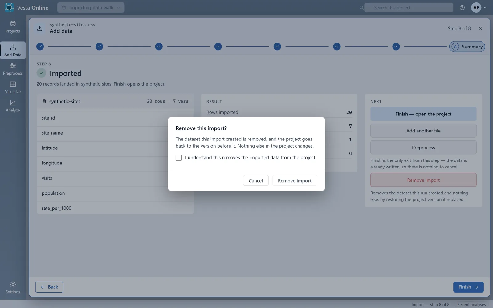
- Remove an importOn the Summary, Remove import asks first: a dialog explains that the dataset this import created is removed and the project goes back to the version before it, and requires you to tick a box before it will go ahead. Cancel keeps the data.
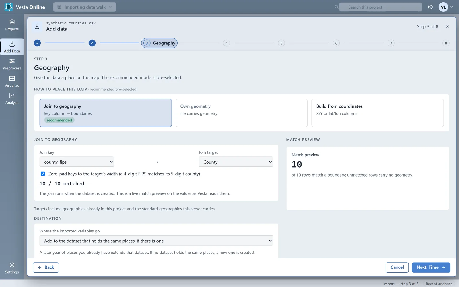
- Join a table to countiesFor a table with an identifier column rather than coordinates, choose Join to geography on the Geography step. Pick the join key column (here county_fips) and a join target (County). Vesta shows how many rows match the boundaries before anything runs.
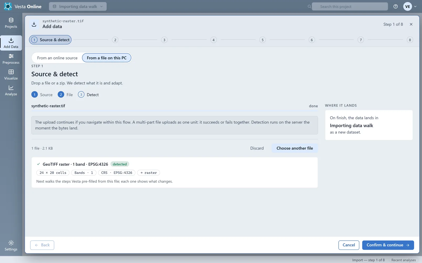
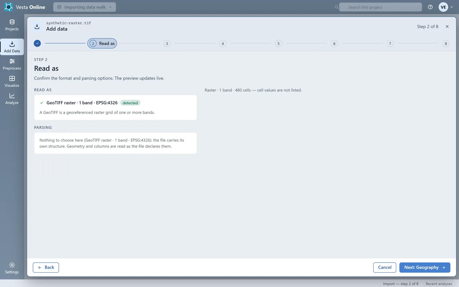
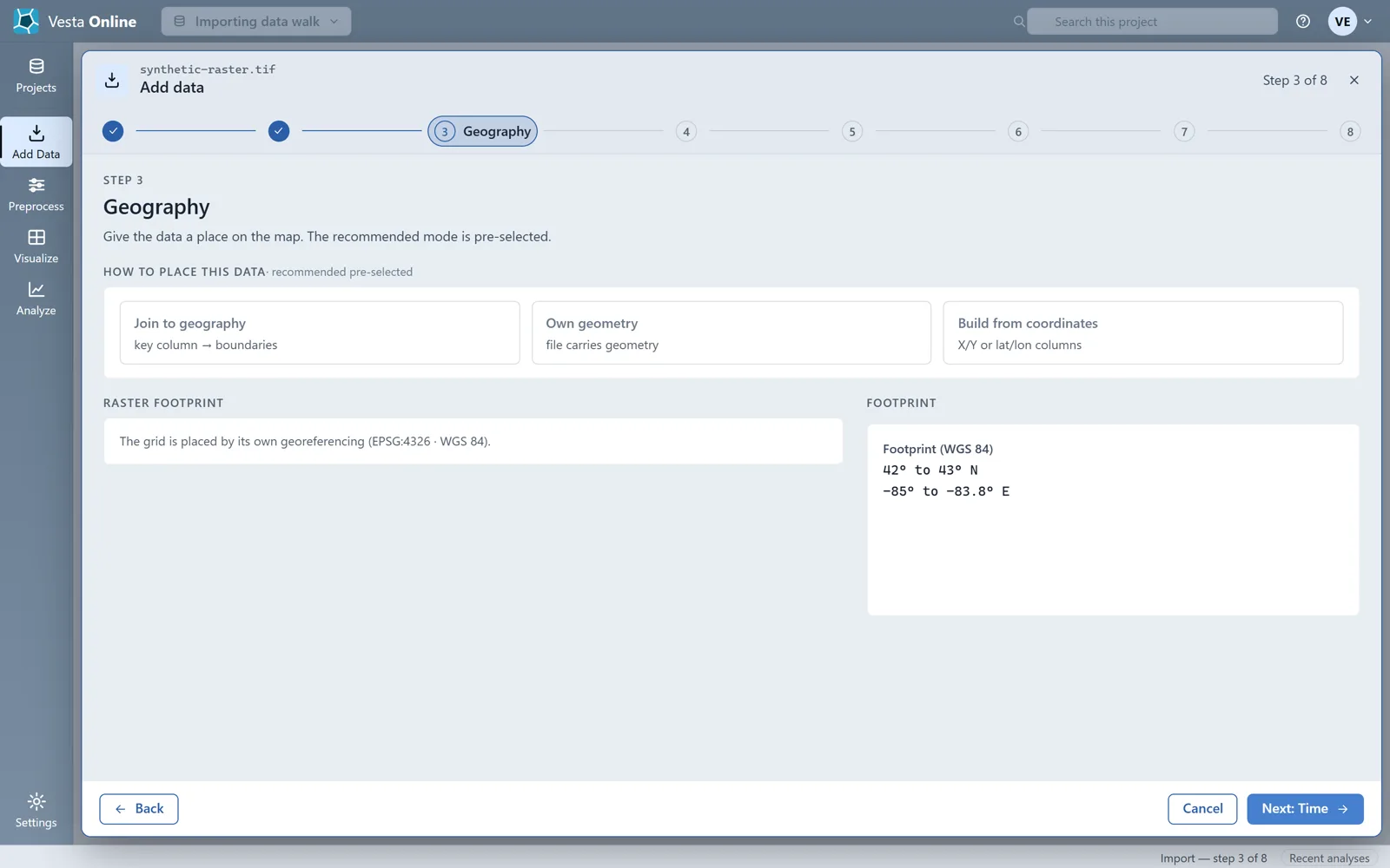
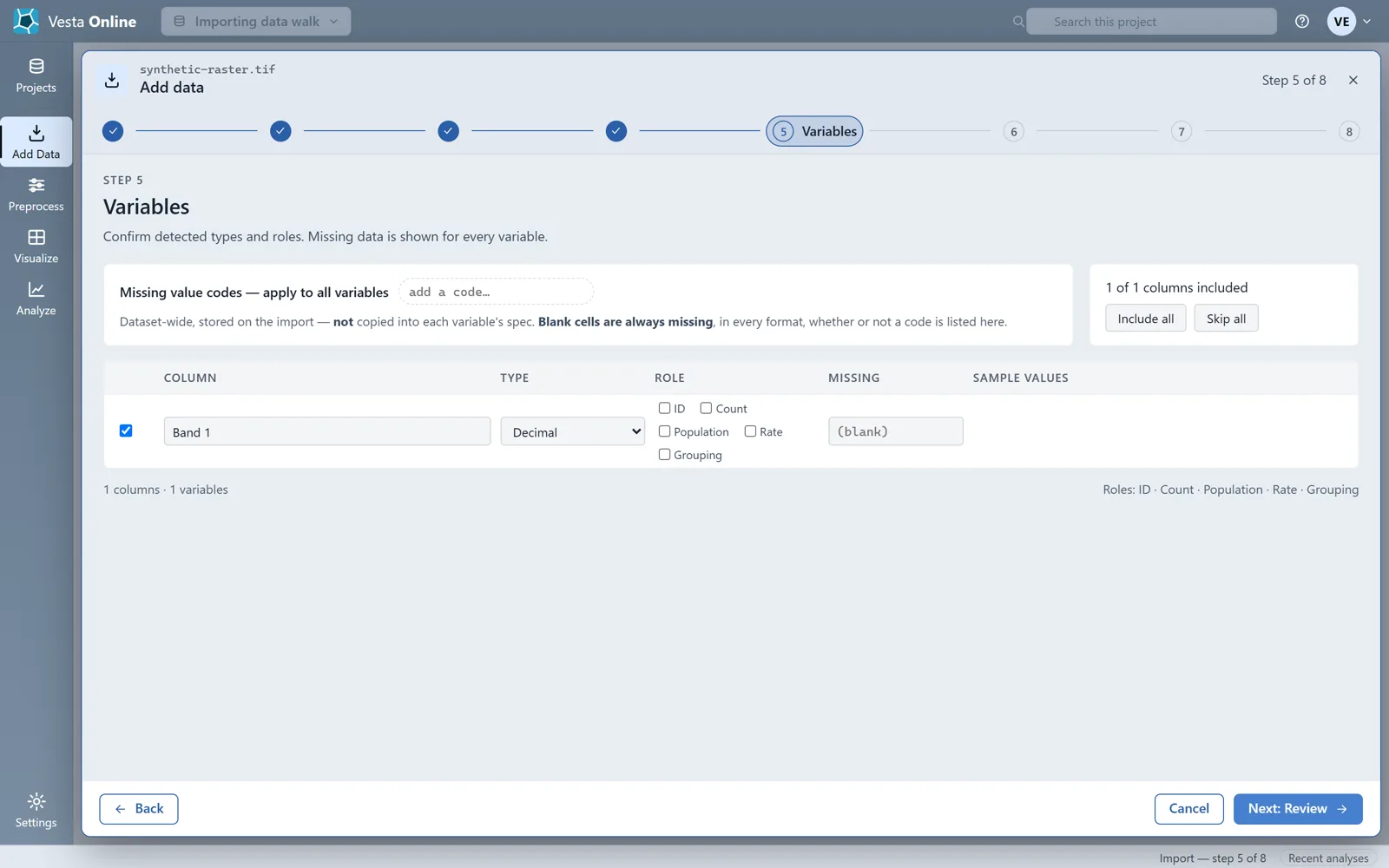
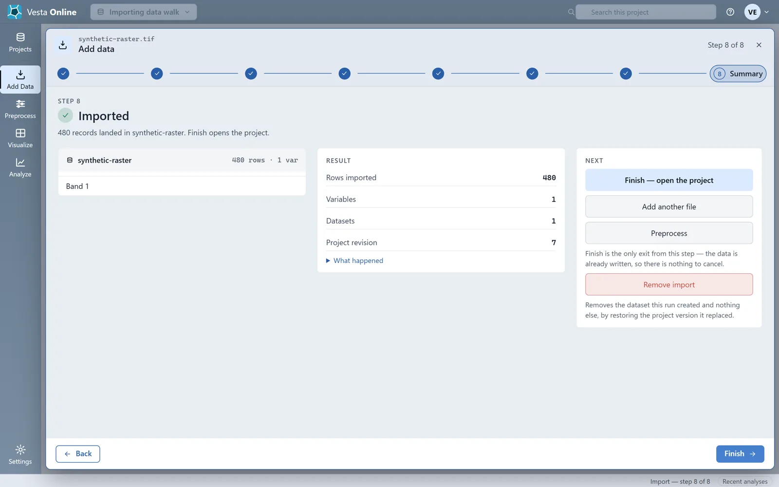
- Import a GeoTIFFChoose From a file on this PC and drop a .tif file, or a .zip that holds it with its sidecars. Vesta Online reports a GeoTIFF raster with its band count, coordinate system and cell grid (here 1 band, EPSG:4326, 24 × 20 cells). Read as has nothing to choose, because the file carries its own structure. Geography places the grid by its own georeferencing and shows the footprint. Time offers the same three modes, and Variables lists each band as a variable. Run the import: each cell becomes a record, so this 24 × 20 grid landed 480 records in 1 variable.
Source, read as and geography
Section titled “Source, read as and geography”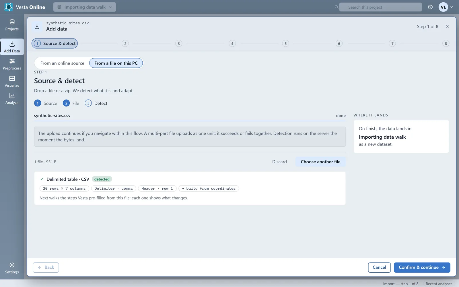
Time, variables and review
Section titled “Time, variables and review”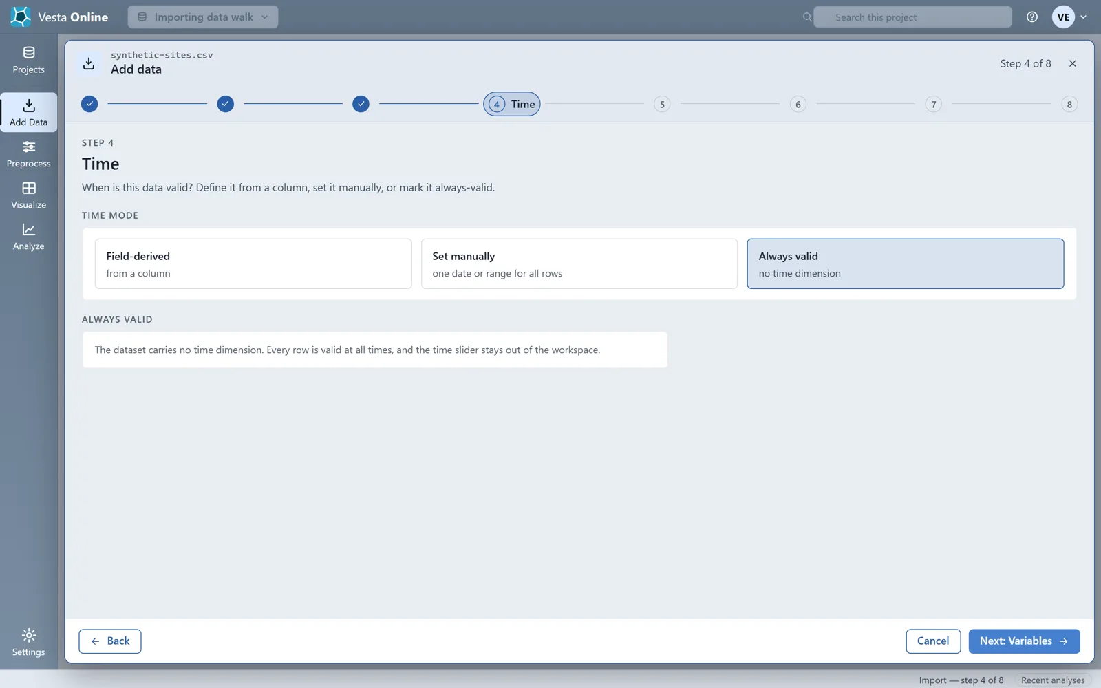
Summary, removing an import and joining
Section titled “Summary, removing an import and joining”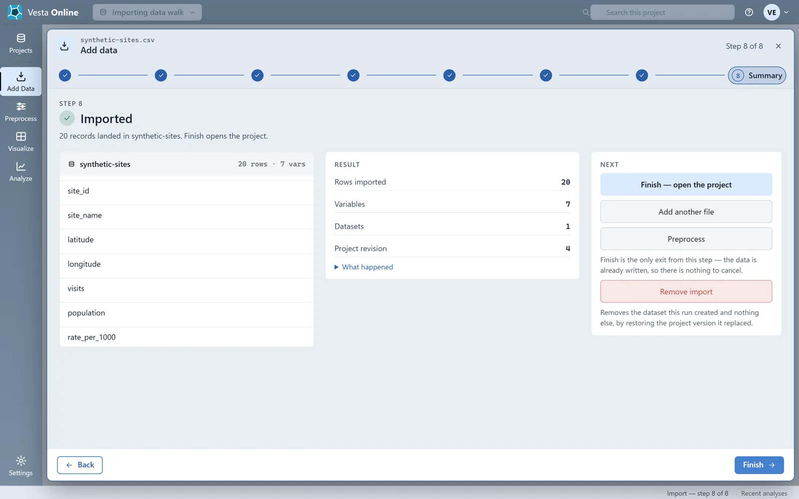
Compute and smooth rates after import
Section titled “Compute and smooth rates after import”Rates are computed after the data has landed, in Preprocess, which opens from the Summary of an import. This walk imports a fourth synthetic file, synthetic-small-counties.csv: 18 Michigan counties with a cases column and a population column, joined to County as in the step above. Every number in it is invented, and seven of the 18 populations are under 100. Every step below was run on Vesta Online.
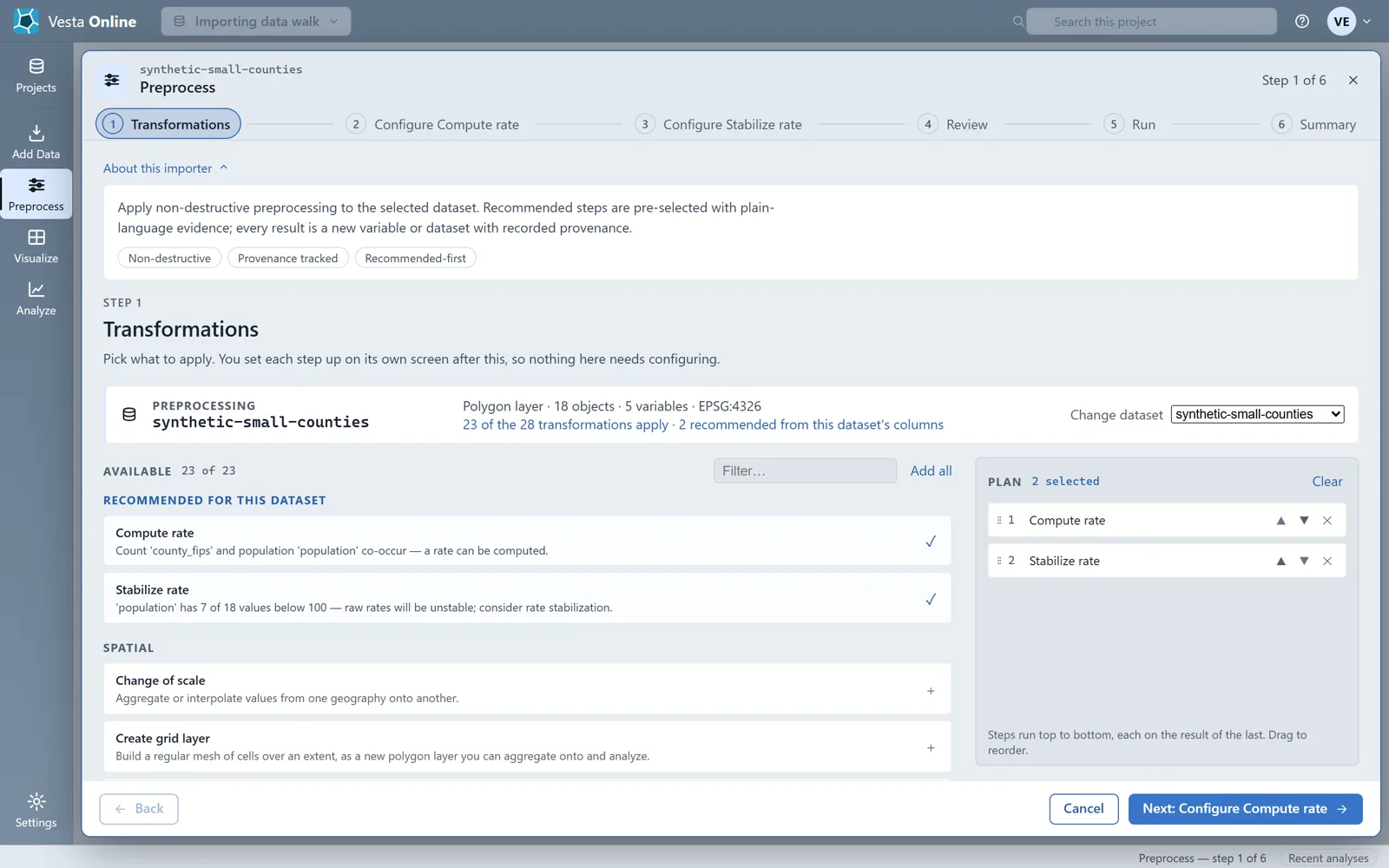
- Open PreprocessImport the file joined to County, as in Join a table to counties above, and run the import: the Summary reports 18 records landed in synthetic-small-counties. Choose Preprocess. It opens on the dataset you just imported. Under RECOMMENDED FOR THIS DATASET it offers Compute rate and Stabilize rate, both already in the plan. The Stabilize rate card gives its reason: 7 of 18 values below 100 in the population column.
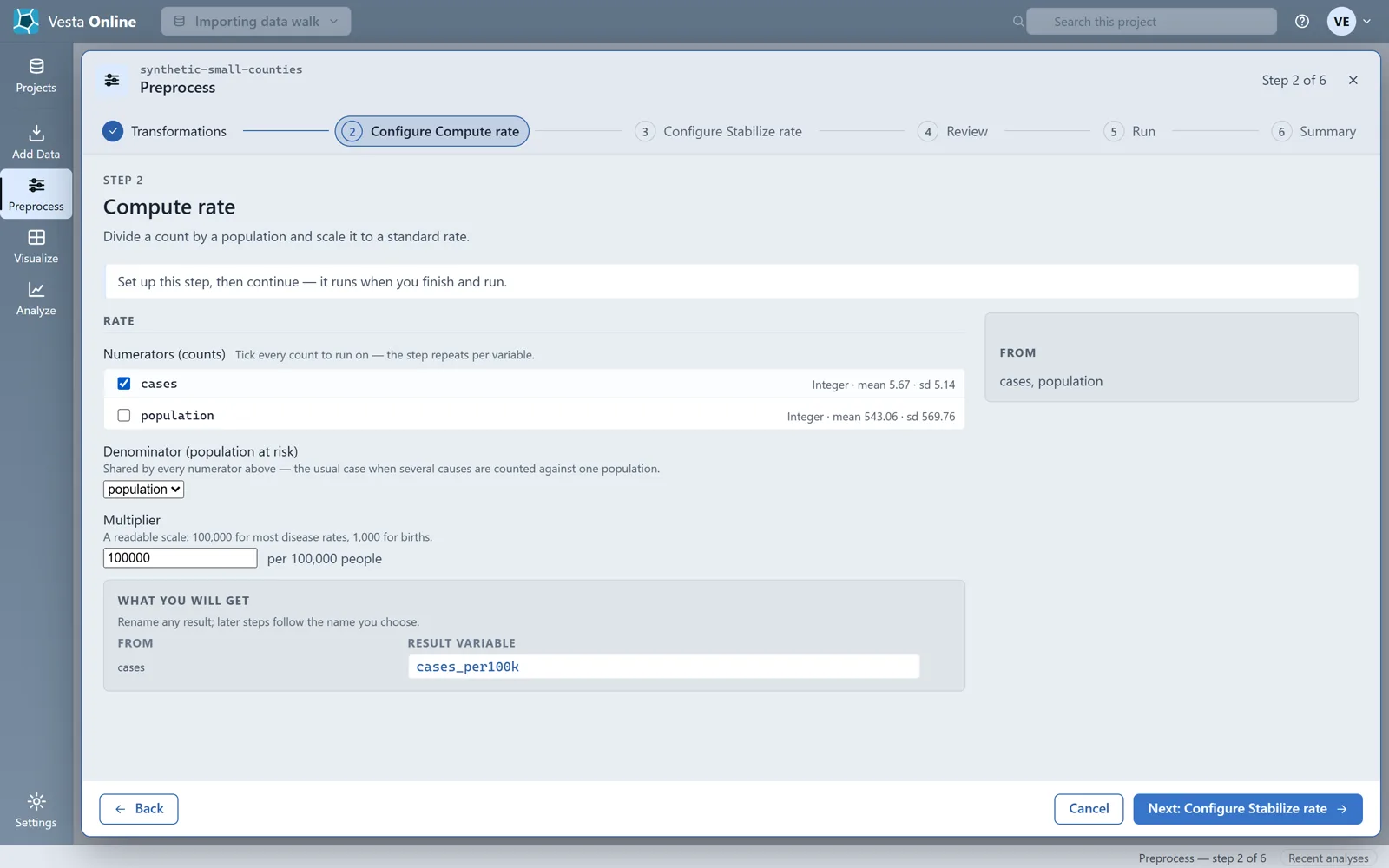
- Compute a rateChoose Next: Configure Compute rate. Tick cases under Numerators (counts) and pick population as the Denominator (population at risk). Multiplier starts at 100,000 and is shown as per 100,000 people. The step names its result variable cases_per100k, and the name can be changed.
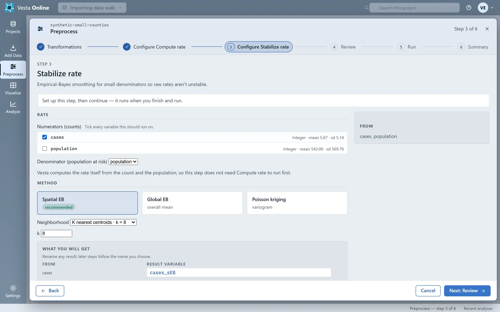
- Smooth the rateChoose Next: Configure Stabilize rate. Tick cases and pick population as the denominator again. Method opens on Spatial EB, marked recommended, with Neighborhood on K nearest centroids and k = 8. The result variable is named cases_sEB. Vesta computes the rate itself from the count and the population, so this step does not need Compute rate to run first.
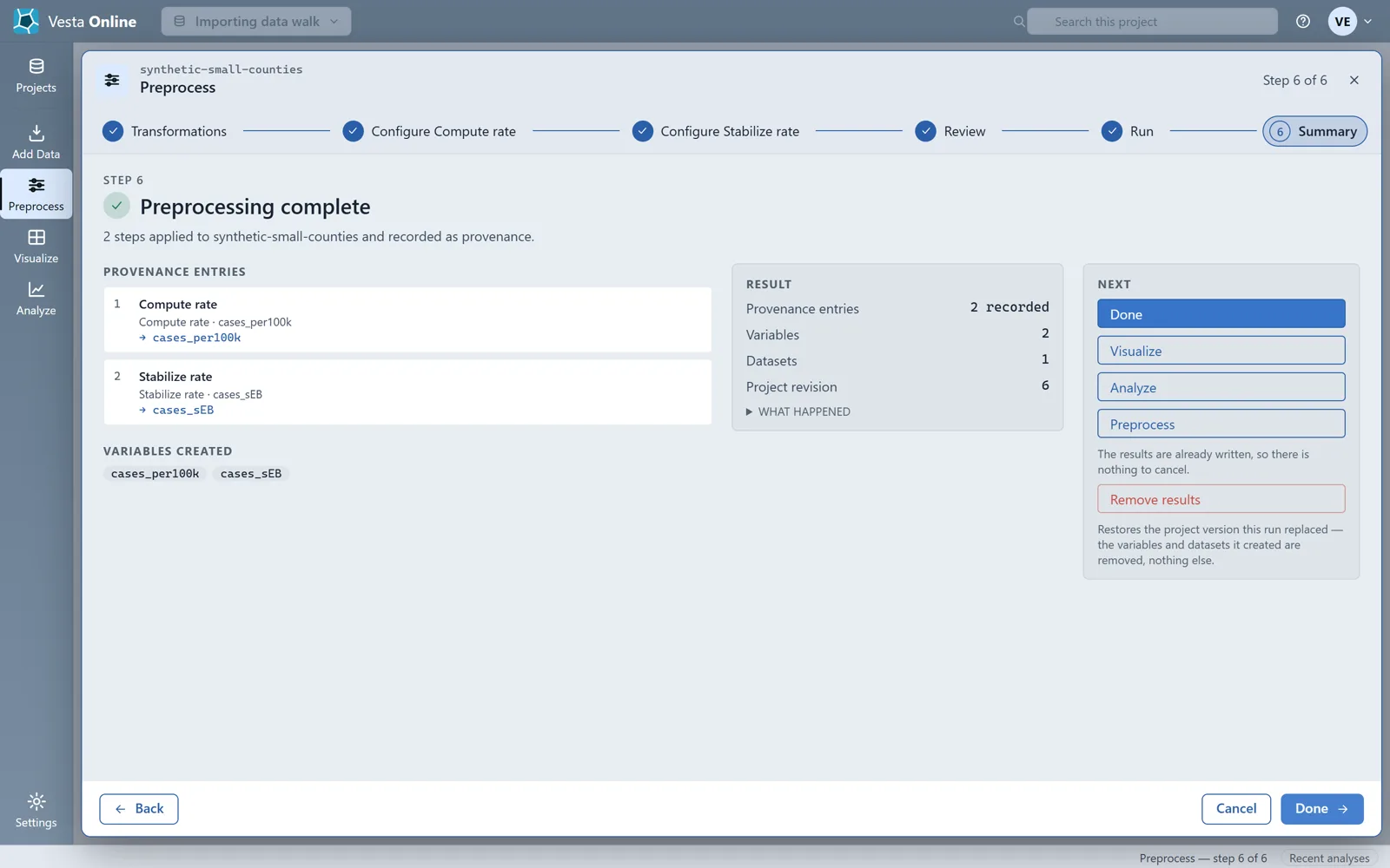
- Run both stepsChoose Next: Review. It says Creates 2 variables: cases_per100k, cases_sEB. Choose Run preprocessing. When the Summary says Preprocessing complete it lists both variables under VARIABLES CREATED. Both are flagged Rate, and cases and population are still in the dataset.
Vesta recommends Stabilize rate when at least 5 percent of the population values are below 100. Read the smoothed rate alongside the raw one, not instead of it: small-denominator areas move a long way and large ones barely move. Stabilize rate runs on vector layers only, so it does not run on a raster such as the GeoTIFF imported above.
If a column already holds a rate, the Variables step can mark its role as Rate.
Supported formats
Section titled “Supported formats”The web importer names these file types: CSV, TXT, XLS, XLSX, shapefile .zip, GeoJSON, KML/KMZ, GeoPackage, GeoTIFF and File Geodatabase (a .gdb folder, zipped). A shapefile has to arrive as one .zip with its .shp, .dbf and .shx files, or as its parts dropped together, and the drop zone takes one dataset per import. This page walks the CSV path and the GeoTIFF path above.
GeoTIFF and File Geodatabase
Section titled “GeoTIFF and File Geodatabase”A GeoTIFF imports as a raster: drop the .tif, or a .zip with its sidecars, and use one raster per import. A File Geodatabase is a folder, so zip the .gdb folder first; Vesta Online reads its first feature class, and a .zip holding more than one geodatabase is refused with a message to upload one per import. The File Geodatabase path was not walked for this page.
Troubleshooting
Section titled “Troubleshooting”| Problem | Fix |
|---|---|
| Rows unmatched on a join | The Geography step shows the match count before the join runs. Check the key column and the join target, and keep the zero-pad option on for FIPS codes that lost a leading zero. |
| A ZCTA import did not narrow to my state | It never does. A ZCTA import covers the whole country. |
| I cannot find the county I want | Counties appears only after you choose its state. Pick the state first, then the county. Leave Counties empty to import every county in the states you chose. |
| Rates look wrong or are missing | Run Compute rate from Preprocess on the import Summary, with a count as the numerator and a population as the denominator. A missing or zero population gives a missing rate, so check those rows first. |
Where next
Section titled “Where next”- Map the imported data and run a first analysis: Quickstart.
- Find clusters in county data: Local cluster analysis.
- Share the project with a colleague: Sharing.