Maps
Change how a Vesta Online map is classified and colored, read its legend and Missing row, switch the basemap and open the layer list.
A map panel draws a dataset’s values on its geography and changes as you change its settings. Every step below was run on Vesta Online, on a copy of the Diabetes and poverty sample project (the copy is made so the sample itself is never edited), and the screenshots come from that run. The map is the share of adults with diagnosed diabetes in each of 3,109 US counties. Changes to a map are saved with the project, so they apply on a project you own.
Change how a map is drawn
Section titled “Change how a map is drawn”- Open a mapOpen a project and choose Focus under the workspace tabs, then click the map's thumbnail in the strip below. This article uses the "Diagnosed diabetes, adults (%), 2022" map on a copy of the Diabetes and poverty sample. Its legend reads 5 classes, Natural Breaks, with a Missing row at the foot.
- Open Map settingsChoose Map settings › at the foot of the legend. A Map Settings sheet opens inside the panel, marked LIVE. It has a Scheme type, a Classification menu, a Classes stepper, a histogram of the values, a color ramp picker and a table of the class breaks.
- Choose a classification methodOpen the Classification menu. It offers Equal Interval, Natural Breaks, Quantile and Standard Deviation. Choose Quantile. The legend and the map redraw with classes that hold about the same number of counties each.
- Set the number of classesChoose + beside Classes to add a class, or − to remove one. Add two and the map has 7 classes. The legend, the histogram and the break table all follow.
- Pick a color rampOpen the ramp menu under the histogram and choose Blues. The legend, the histogram bars, the break table and the map all take the new colors.
- Read the legendChoose Done to close the sheet. The legend shows each class with its range and the number of counties in it, and a Missing row at the foot.
- Choose a basemapChoose the basemap button to open the Basemap list. Type in the Filter styles box to narrow it, and choose a style. This walk chose Satellite, and the data stayed on top of the imagery.
- Open the layer listChoose the Layers button under the zoom control to open the Layers list. It shows one row per layer, with a visibility box and buttons to move, reset and remove the layer.
Your changes are kept
Section titled “Your changes are kept”The walk made its changes one after another, without pausing between them, then reloaded the project. The classification method (Quantile), the 7 classes, the Blues ramp and the Satellite basemap were all still set, and the workspace opened in the same Focus layout.
What you should see
Section titled “What you should see”The map
Section titled “The map”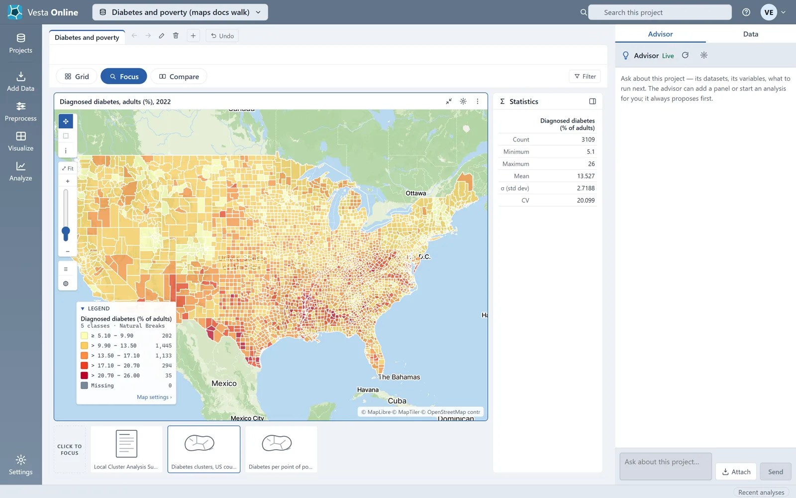
Map Settings
Section titled “Map Settings”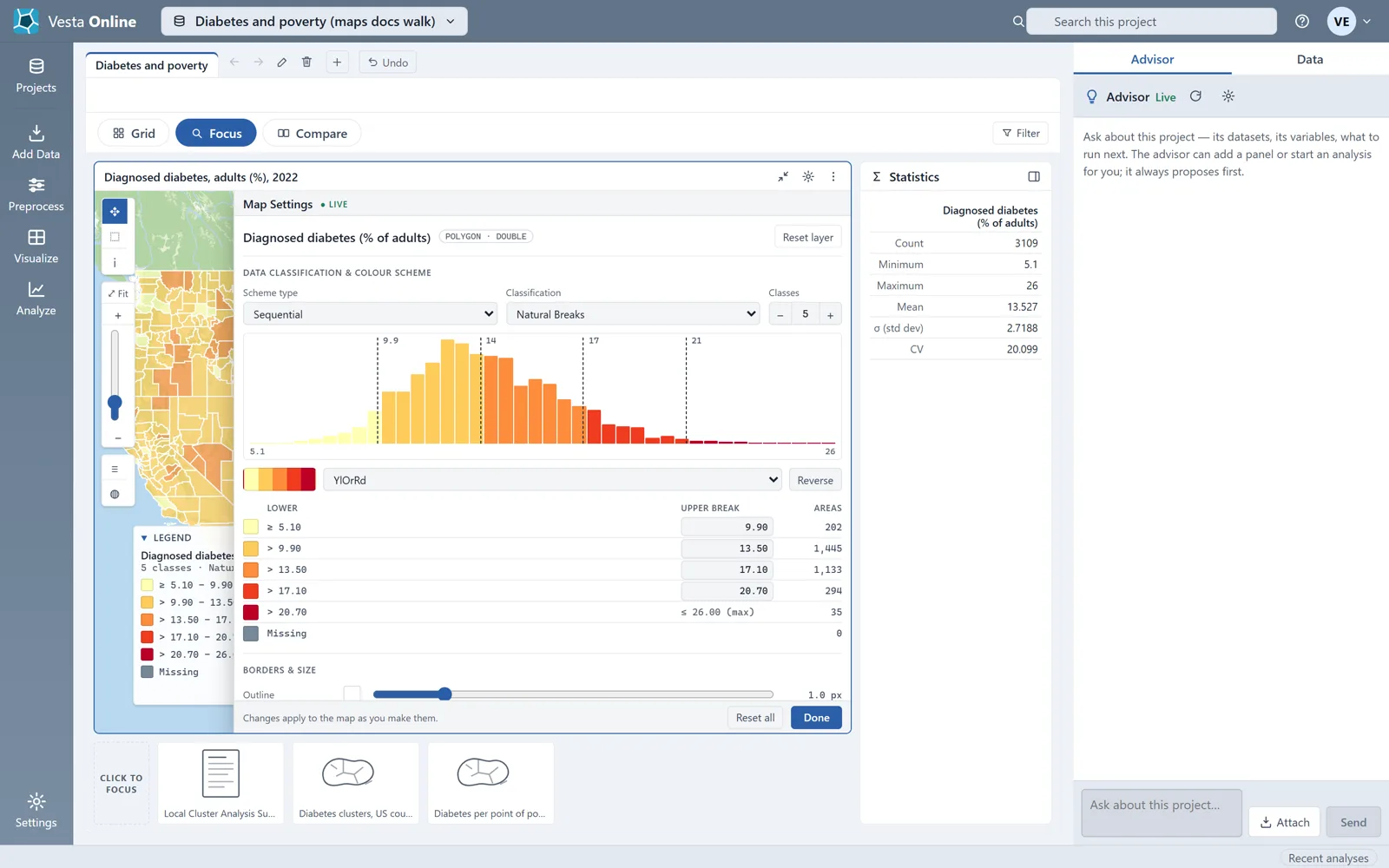
Quantile
Section titled “Quantile”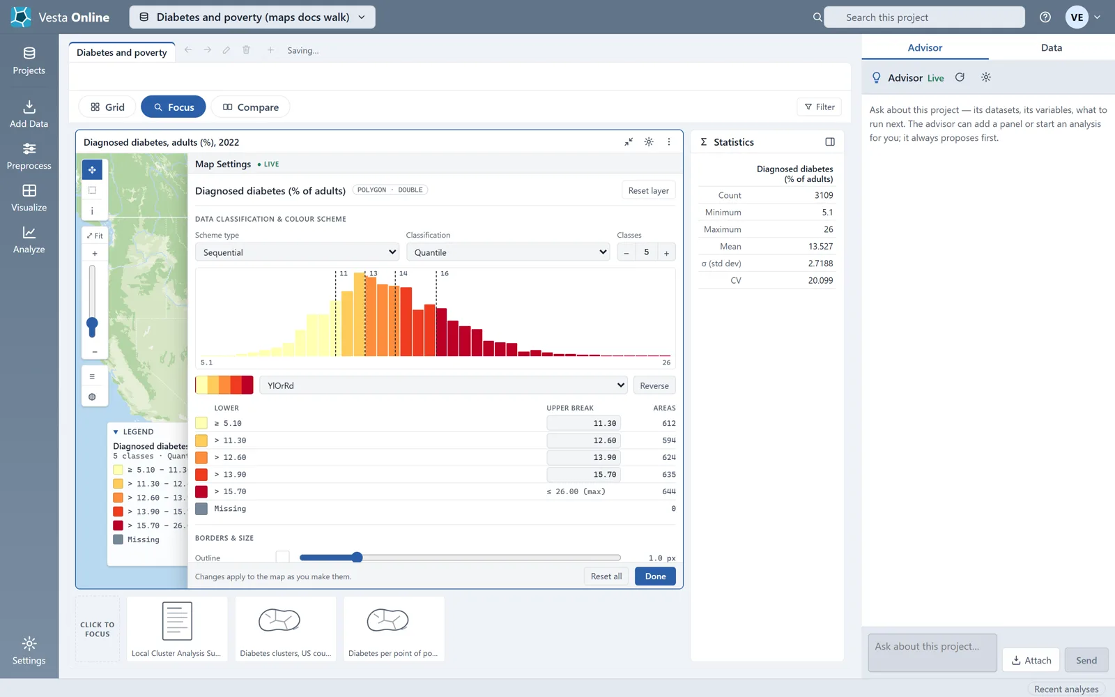
7 classes
Section titled “7 classes”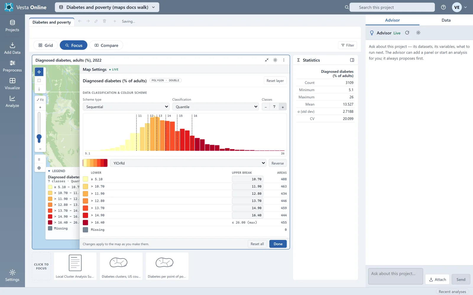
Blues ramp
Section titled “Blues ramp”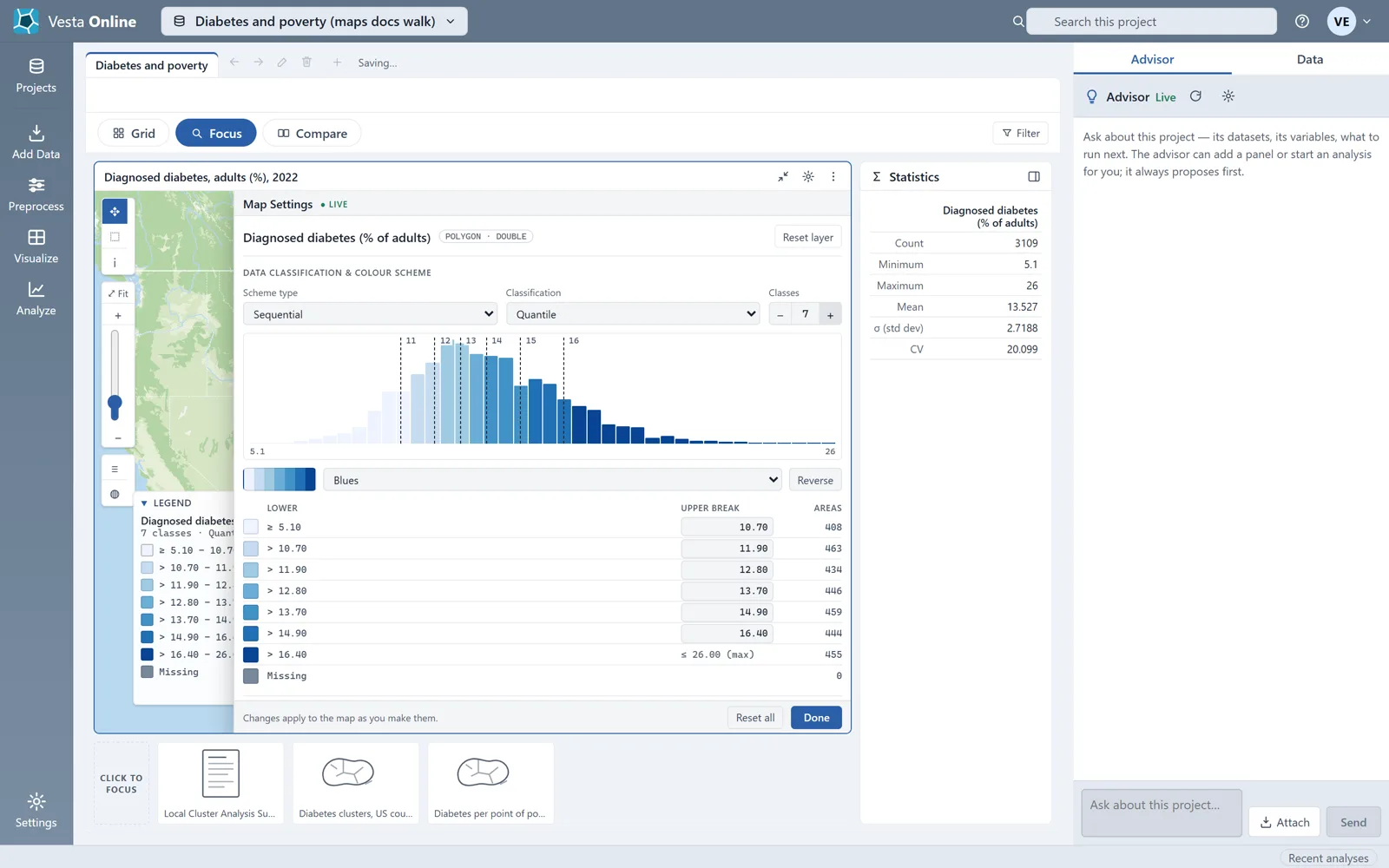
The legend
Section titled “The legend”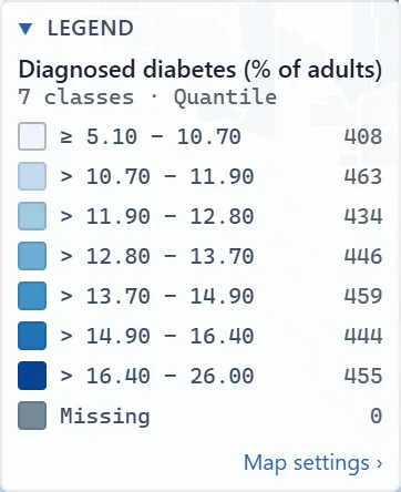
Satellite basemap
Section titled “Satellite basemap”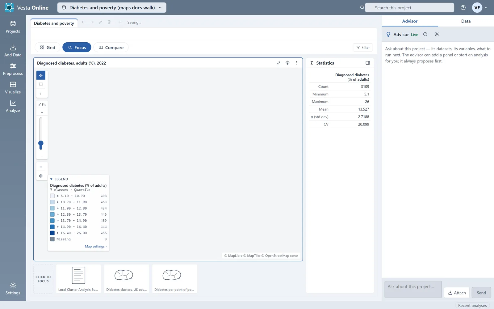
Layers
Section titled “Layers”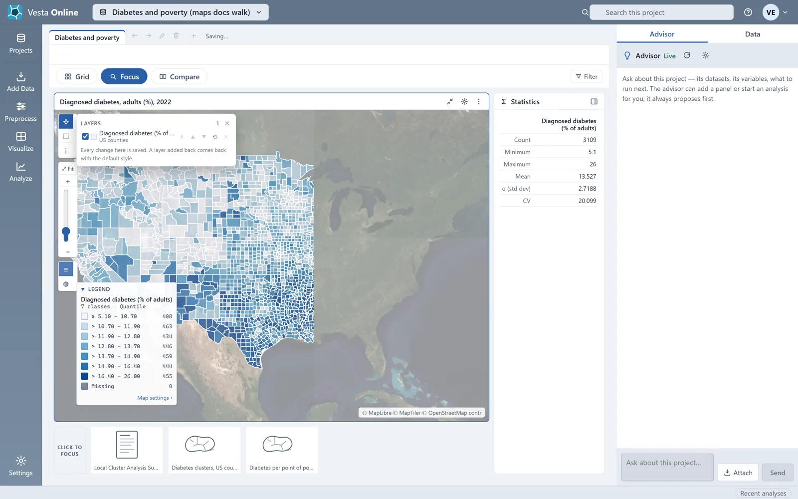
Classification methods
Section titled “Classification methods”| Choice | What it does |
|---|---|
| Natural Breaks | The map opened on this method. It gave 202, 1,445, 1,133, 294 and 35 counties in the five classes. |
| Quantile | Puts about the same number of counties in every class, so no class is nearly empty. |
| Equal Interval | In the menu, not run for this article. |
| Standard Deviation | In the menu, not run for this article. |
The Classes stepper goes from 2 to 9 classes. The Scheme type menu also offers Diverging and Qualitative; those were not run. If you edit an upper break in the table, the method changes to Custom.
The legend
Section titled “The legend”The legend lists each class with its range and its count. The Missing row is always shown, even when it counts zero. A class that no county falls in at any time step is left out of the legend. When a panel is narrow the legend starts folded; choose its header to open it. Map settings › at its foot opens the sheet.
Basemaps
Section titled “Basemaps”The Basemap list holds 16 styles, with Base as the current style when a map opens. Choosing Satellite on one map makes every map in that tab satellite. The attribution line at the lower right of the map credits MapLibre, MapTiler and OpenStreetMap contributors.
Layers
Section titled “Layers”The Layers list holds one row per layer. The buttons on each row move the layer up or down (▲ and ▼), reset its style, or remove it (✕). In this project each map has a single layer, so ▲, ▼ and ✕ are dimmed. The tooltip on ✕ reads “A map keeps at least one layer”, and the one on ▲ reads “Move up (draw later)”. The note at the foot of the list says “Every change here is saved.”
A map whose data changes over time follows the workspace time slider. See The workspace for the slider.
Where next
Section titled “Where next”- See the panels around a map: The workspace.
- Make a map from an analysis: Local cluster analysis.
- Bring in your own data: Importing data.