Preparing data
Get a dataset ready for analysis: keep join keys as text, rename and remove variables, and run Change of scale and Join layers in Preprocess.
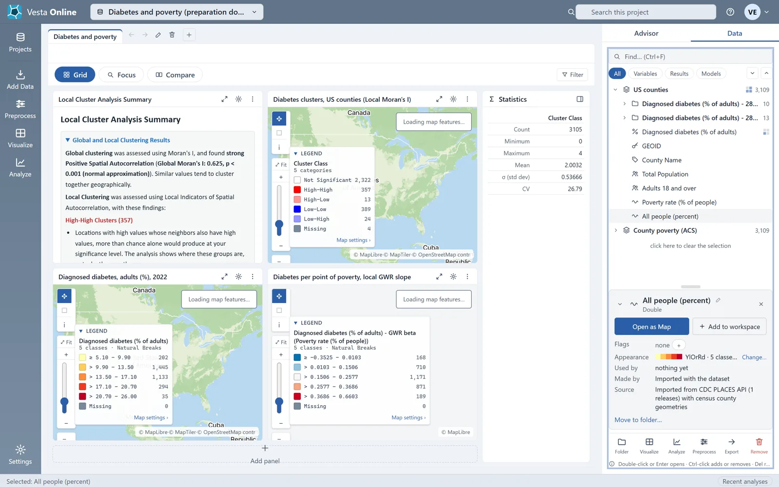
Most of the work of preparing data happens before it reaches Vesta Online, and a little happens after. This article covers both: what your file needs before import, and what you can do to a dataset that is already in a project (rename a variable, remove one, and run Preprocess steps). The walk uses a copy of the Diabetes and poverty sample, which holds two datasets, US counties and County poverty (ACS), each with 3,109 counties. Every step below was run on Vesta Online, and the screenshots come from that run. For the import steps themselves, see Importing data.
Before you import
Section titled “Before you import”One thing has to be right in your file, because the import wizard will not fix it for you.
Rates can wait until after import. If your file has a count and a population, Preprocess can compute the rate and smooth it: see Compute and smooth rates after import in Importing data. If your file already has a column that holds a rate, that is fine. The Variables step can mark that column’s role as Rate.
Keep join keys as text. A code such as a county FIPS is a fixed-width digit code, so it types as String. As a number, 06037 becomes 6037 and matches nothing. When you join a table to geography, the import wizard says this itself and locks the key column to String, with an explicit Unlock.
Prepare a dataset in a project
Section titled “Prepare a dataset in a project”- Open the Data panelOpen the project and choose the Data tab on the right. Each dataset is a row; expand US counties to list its variables, with an icon for each variable's type.
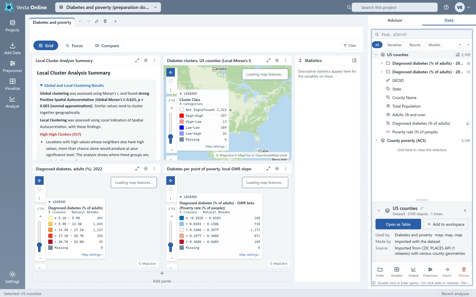
- Rename a variableSelect a variable, press F2, type the new name and press Enter. Here Total Pop 18+ becomes Adults 18 and over. Vesta shows a confirmation, Renamed to Adults 18 and over, with an Undo button, and the new name is still there when you reload the project.
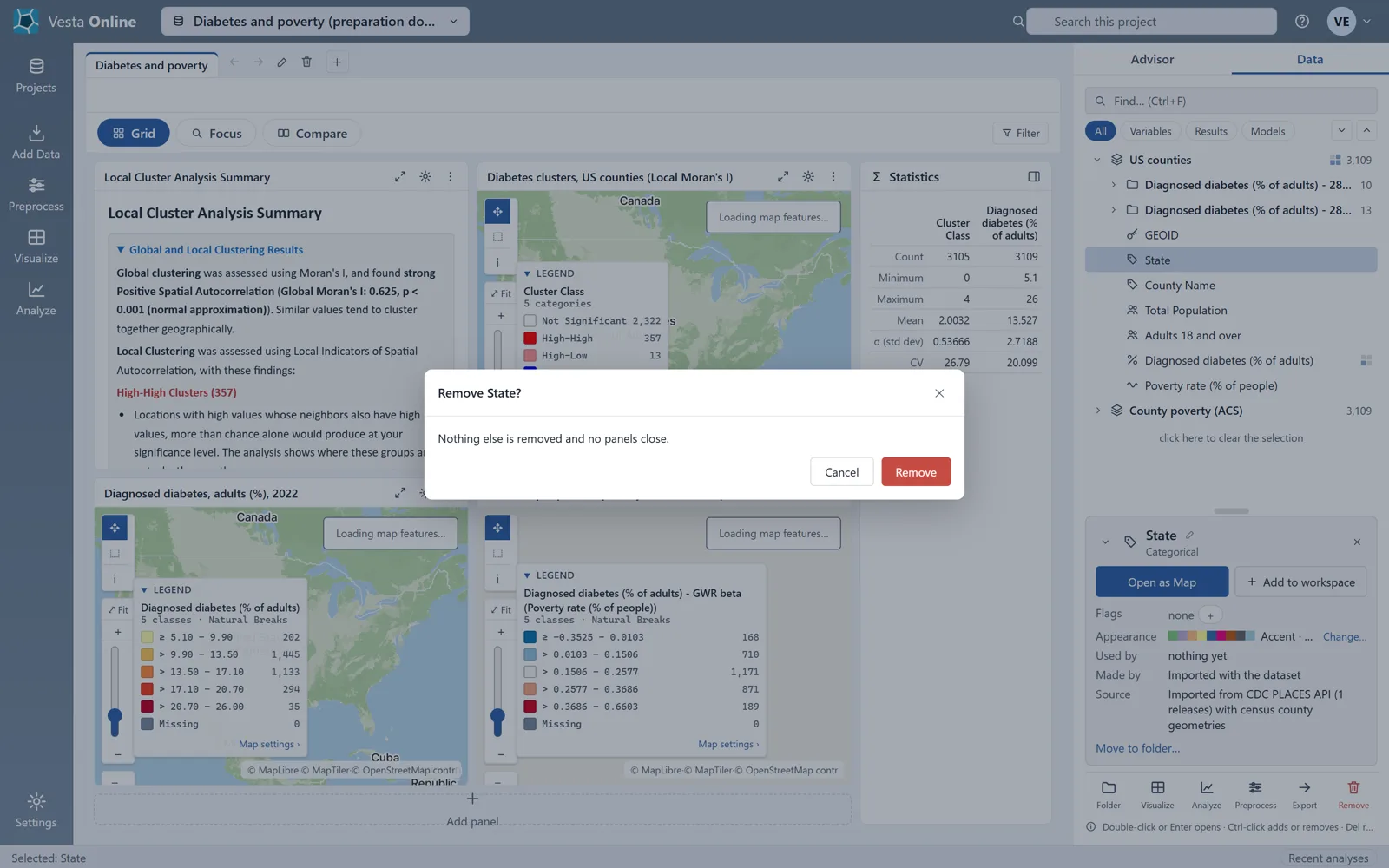
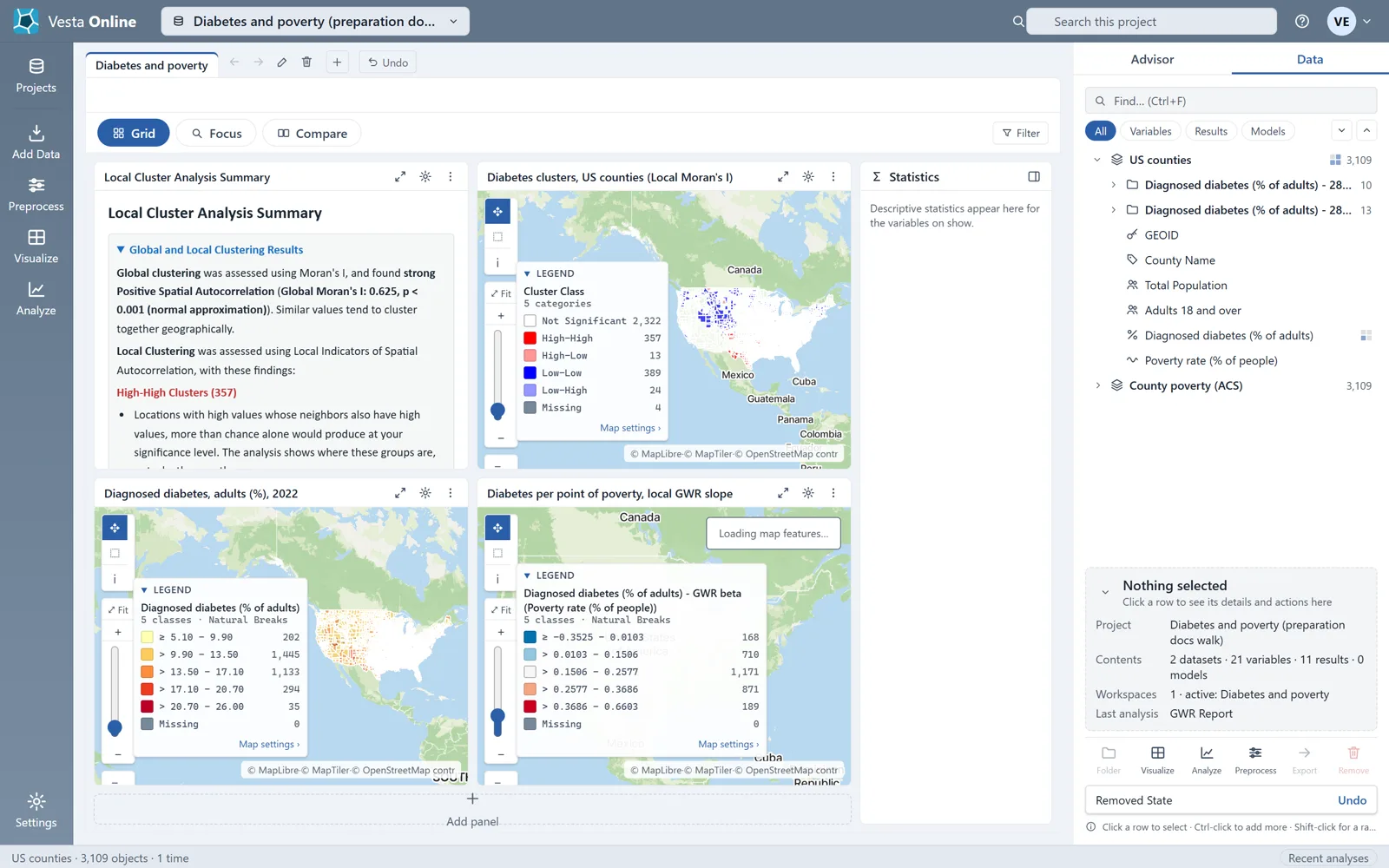
- Remove a variableSelect a variable and choose Remove at the bottom of the card. A dialog asks Remove State? and says that nothing else is removed and no panels close. Choose Remove to confirm, or Cancel to keep it. The variable leaves the list.
- Choose Change of scaleChoose Preprocess in the left rail, then pick the dataset under Change dataset (here County poverty (ACS)). Preprocess opens at Transformations, a plan of the steps to run in order. Clear the plan if it holds steps you do not want, then choose Change of scale, which aggregates or interpolates values from one geography onto another.
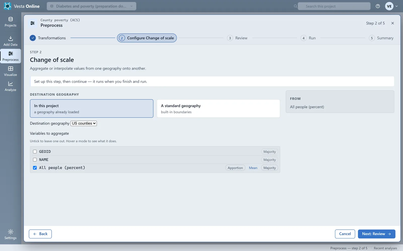
- Set up the stepChoose Next: Configure Change of scale. Under Destination geography keep In this project and pick US counties. Untick the variables you do not need (here GEOID and NAME) and choose a method for the one you keep: Apportion, Mean or Majority. This walk uses Mean on All people (percent).
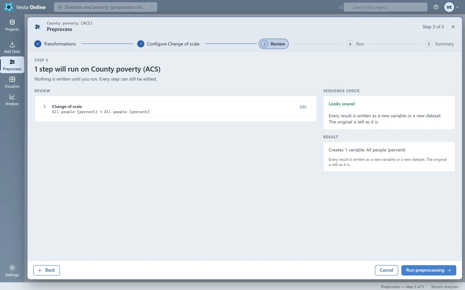
- Review the planChoose Next: Review. Review lists the step with its variable and states that nothing is written until you run.
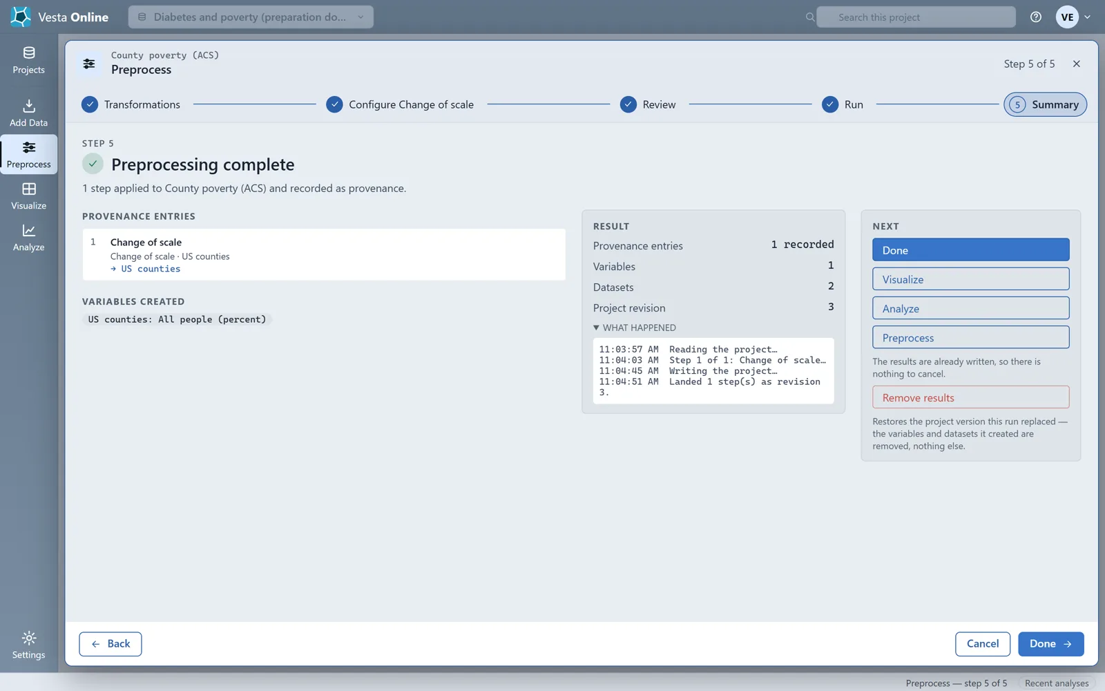
- Run it and read the SummaryChoose Run preprocessing. The run is a server job with a log; when it finishes the Summary says how many steps were applied and records them as provenance. The Next panel offers Done, Visualize, Analyze and Preprocess, and Remove results, which restores the project version the run replaced.
- Find the new variableChoose Done and expand US counties in the Data panel. The aggregated values are a new variable on US counties, here All people (percent), a Double, with State already gone from the earlier step.
- Choose Join layersBack in Preprocess, with US counties as the dataset, clear the plan and choose Join layers. After Next: Configure Join layers, pick the Source layer (here County poverty (ACS)) and a key on each side (GEOID and GEOID). The zero-pad option rewrites numeric keys, for example 5095 to 05095; leave it unticked for keys that are already text. Unmatched rows are kept (left outer) or dropped (matched rows only).
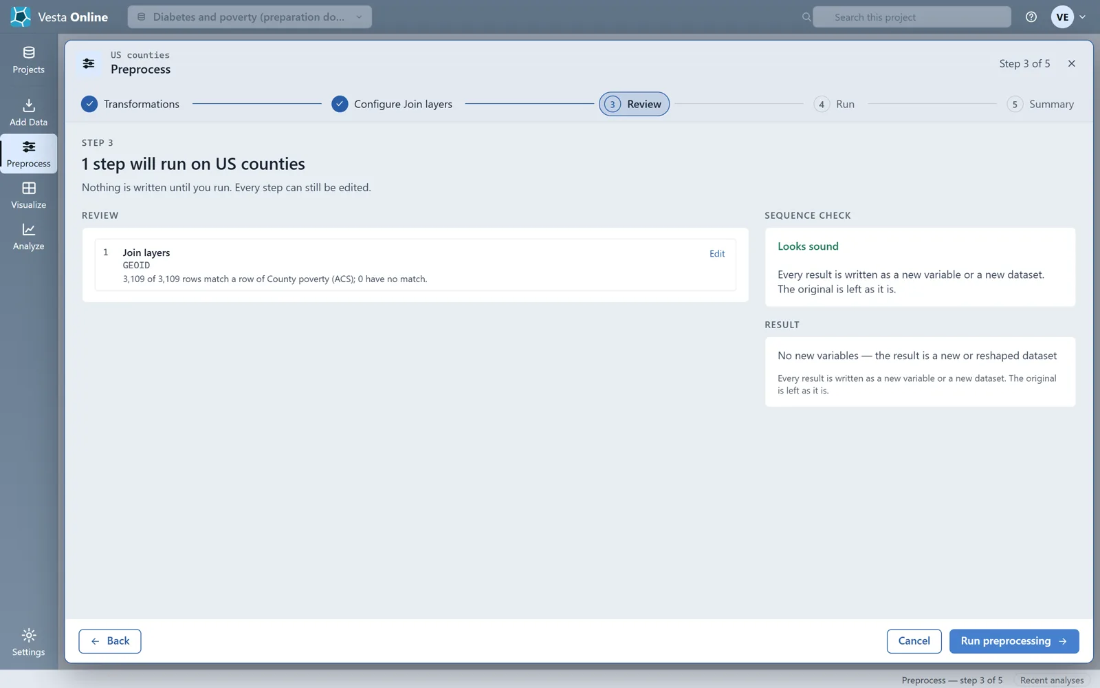
- Review the joinChoose Next: Review. This run stopped here, without running the join.
What you should see
Section titled “What you should see”In the Data panel
Section titled “In the Data panel”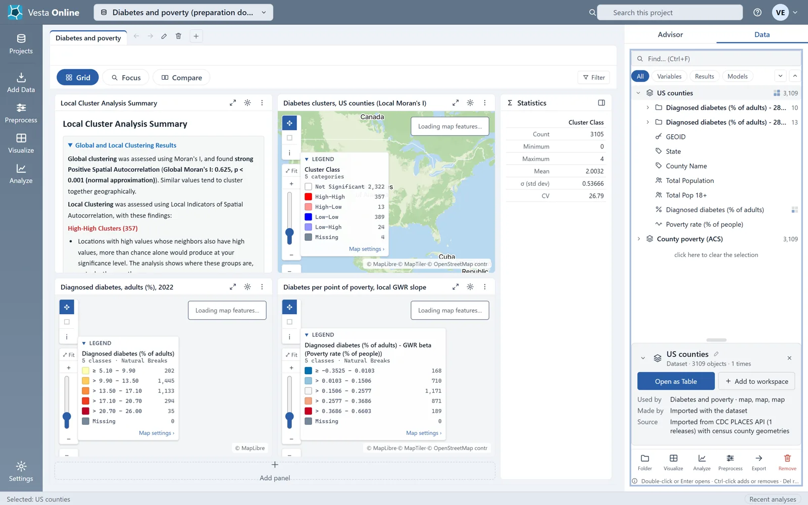
Change of scale
Section titled “Change of scale”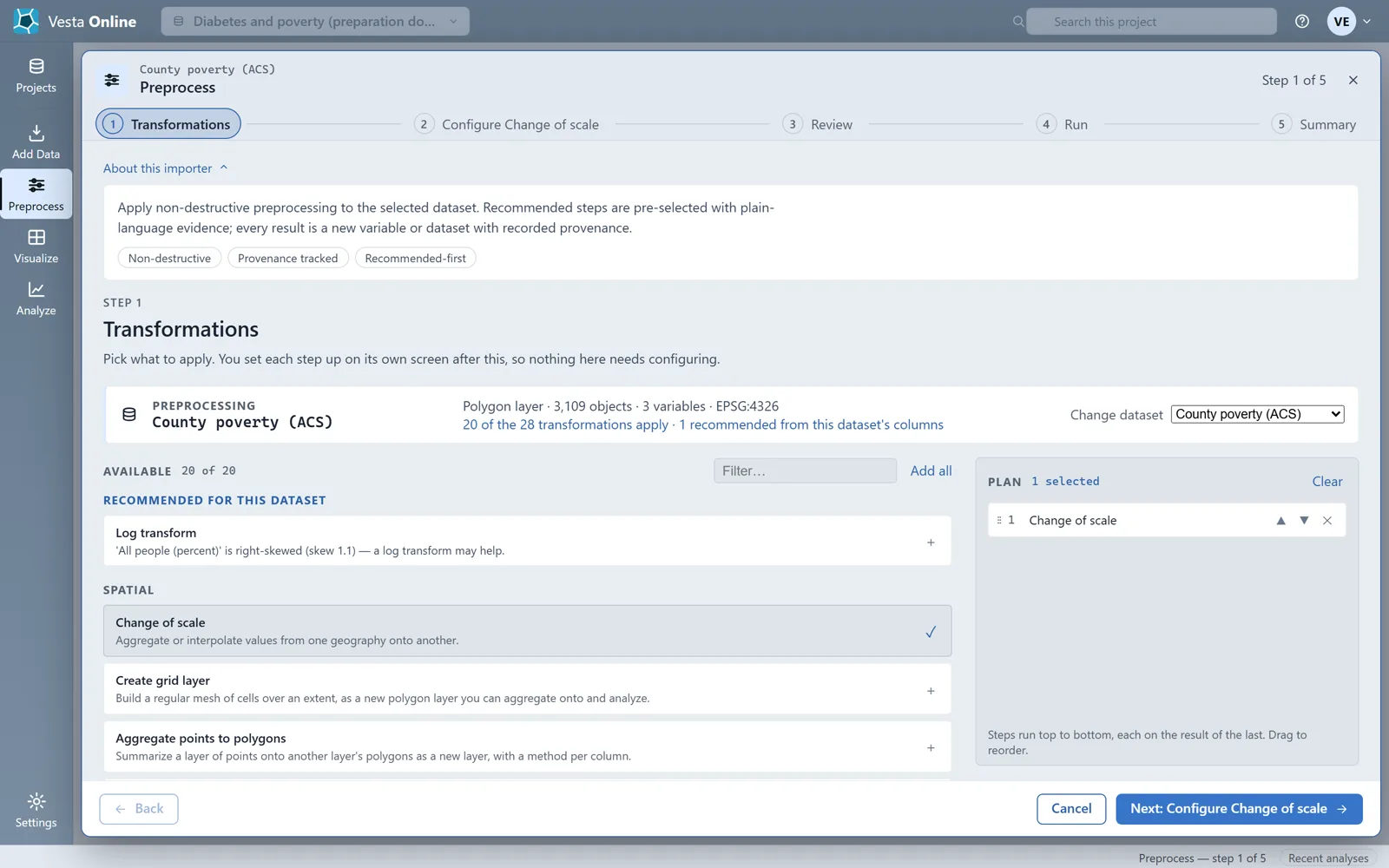
Join layers
Section titled “Join layers”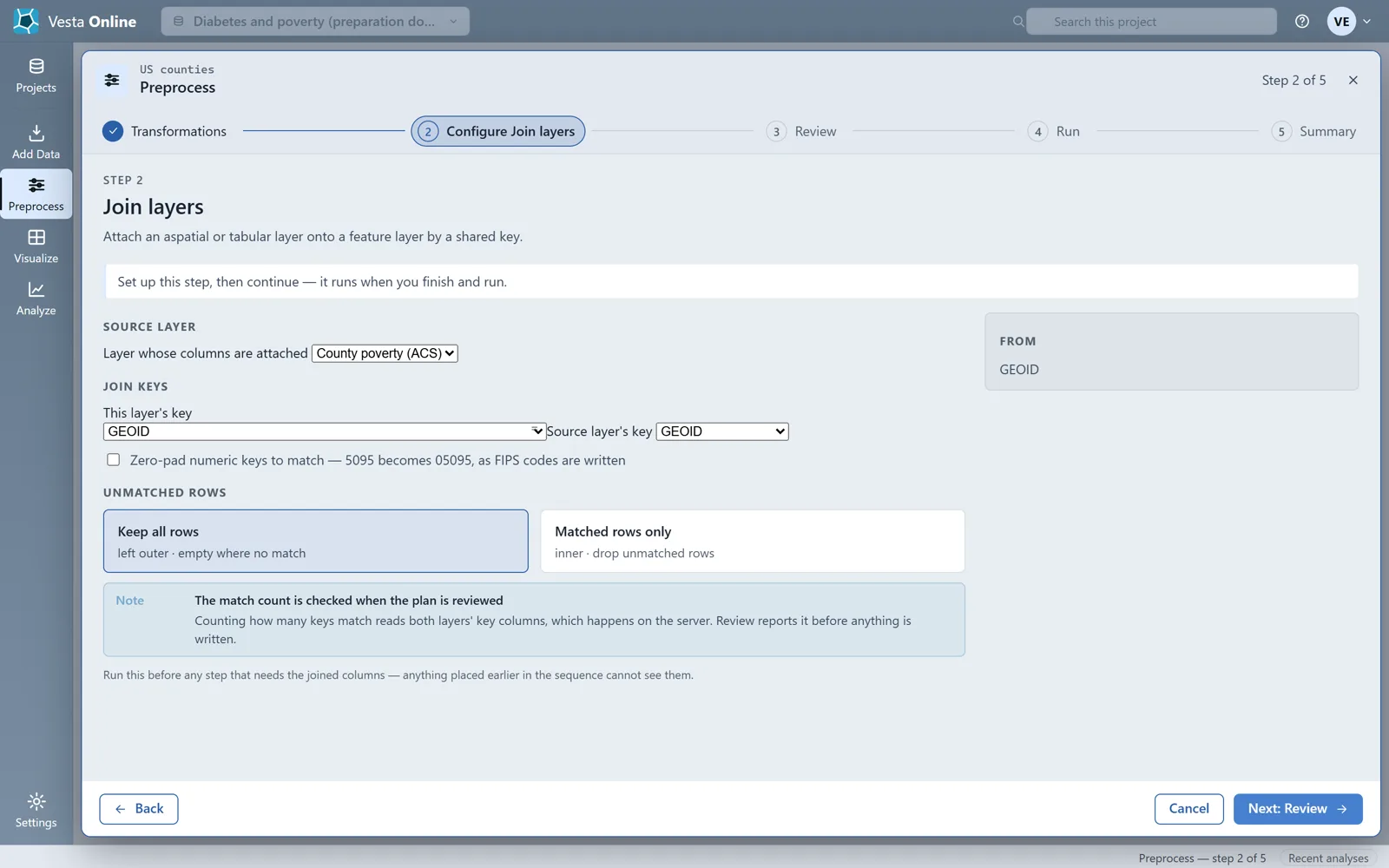
Two ways to put a table’s values on a geography
Section titled “Two ways to put a table’s values on a geography”Change of scale moves values from one geography onto another, and Join layers attaches a table to a layer by a shared key. They overlap when two datasets share the same geometry, as the two datasets here do. Use Change of scale when the geographies differ, and Join layers when you have a table keyed by an identifier. The walk ran Change of scale only; a Join layers run would add a second copy of the poverty column, so it stopped at Review.
What Preprocess does to your data
Section titled “What Preprocess does to your data”For the steps walked here, Review says: “Every result is written as a new variable or a new dataset. The original is left as it is.” A step that replaces its original dataset shows a different note, “One step replaces the original dataset. That cannot be undone once it has run.”, and a Not undoable badge. Change of scale, as walked here, showed the first note. Removing a variable is different: the variable leaves the dataset, and Undo is the way back.
Where next
Section titled “Where next”- Bring data in, including rates and join keys: Importing data.
- Run a first analysis on the prepared data: Quickstart.
- Find clusters in county data: Local cluster analysis.
- Share the prepared project: Sharing.