Local cluster analysis
Find where high or low values cluster, and which areas stand out from their neighbors, with Local Cluster Analysis in Vesta Online.
Local Cluster Analysis compares each area’s value with its neighbors’ and reports where high values sit among high values, low among low, or one value stands out against its surroundings. This article runs it on diagnosed diabetes (% of adults) for the 3,109 US counties in the Diabetes and poverty sample. Every step below was run on Vesta Online, and the screenshots come from that run. For a shorter first run with the defaults, see the Quickstart.
The seven steps
Section titled “The seven steps”- Open a project that holds your dataOpen the Projects page, select a project and choose Open Project. This walk-through uses a copy of the Diabetes and poverty sample, whose US counties dataset has 3,109 counties. It tests one variable at a time.
- Choose Local Cluster AnalysisChoose Analyze in the left rail, then Find clusters & hotspots, then Local Cluster Analysis, and choose Pick a method. The analysis has six steps: Analysis, Variables, Spatial weights, Significance, Run and Summary.
- Pick the variableOn Variables choose the dataset, US counties, and the variable, Diagnosed diabetes (% of adults). Objects with a missing value are left out of the analysis, not treated as zero. Choose Next: Spatial weights.
- Set the neighborsThe step asks what counts as a neighbor. Leave the definition on Detect: a grid uses its cells, point data uses nearest neighbors, polygons use shared boundaries. For counties it reports Shared boundary adjacency. The Guidance switch at the top right sets how much the step shows; Full control also shows Neighbors per object (1 to 50, used by k nearest weights and by point data; a value outside the range is set to the nearest end and a note says so, for example "51 is outside the allowed range (1 to 50); using 50."), Distance band (map units; it applies only to Distance band weights and is ignored with any other neighbor definition), Use rook contiguity (queen is the default) and Row-standardize the weights (on by default). Choose Next: Significance.
- Set the significanceAlpha is the cutoff for calling an object a cluster or outlier; the default is 0.05. Randomizations are the permutations behind each pseudo-p value: the default is 100, the minimum is 99 and the maximum is 9,999. This walk-through uses 199. At Full control you can also choose a multiple-testing correction, None, False discovery rate (Benjamini-Hochberg) or Bonferroni, and a seed. Leave the seed blank for a new one on every run, or set it (here 12345) so the run can be repeated. This walk-through uses False discovery rate. Choose Run analysis when you are ready.
- Run the analysisThe run happens on the server: a short run runs directly on the server; a longer one is queued for a compute worker. If you start a second run while another of yours is going, the step says Another analysis of yours is still running. The Summary then lists what was saved and what to check.
- Open the result workspaceChoose Open in workspace. The result workspace has a cluster map, a category histogram, a Moran scatterplot and the written summary. The map shows Loading map features while it draws.
What you should see
Section titled “What you should see”The method
Section titled “The method”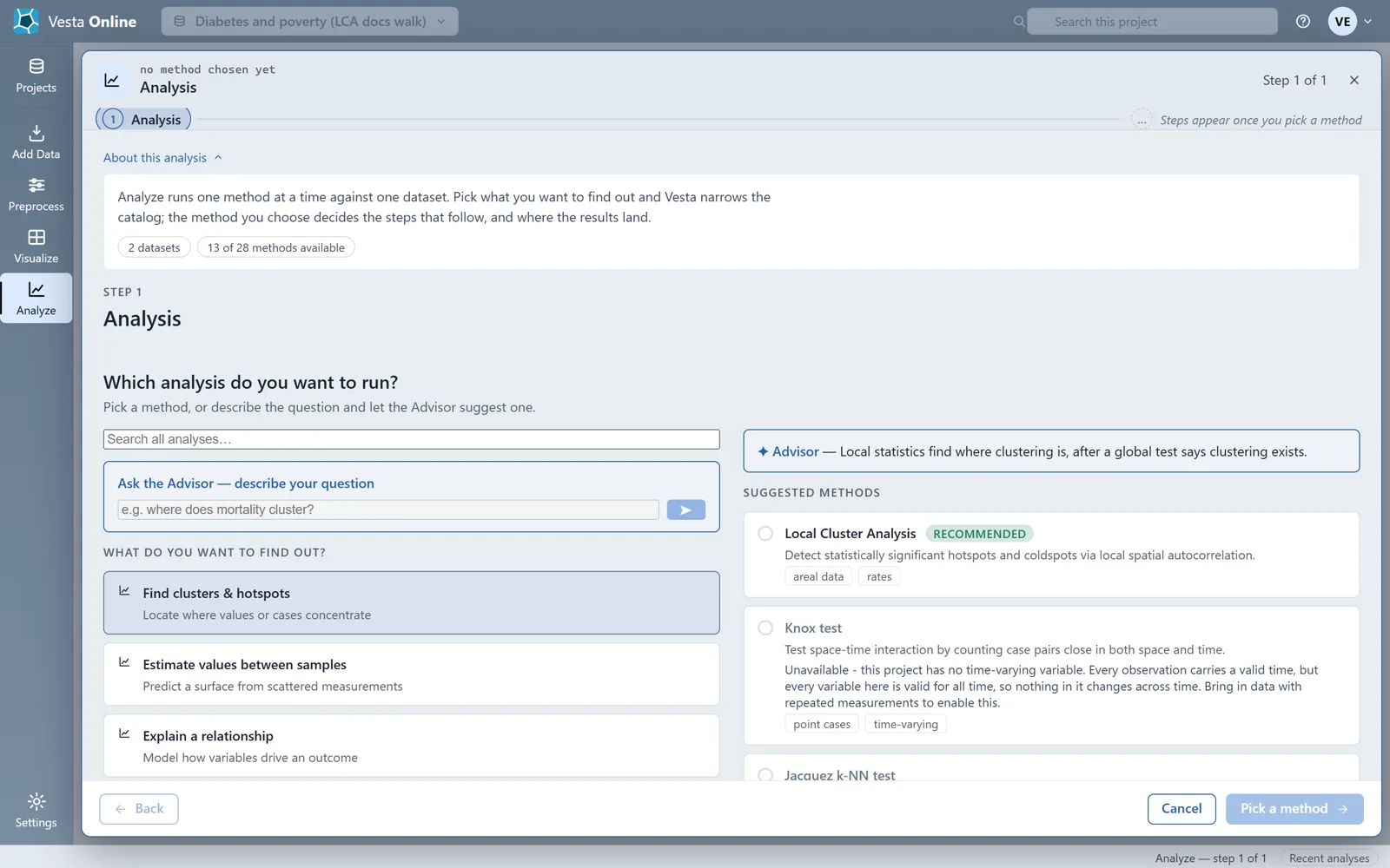
The variable
Section titled “The variable”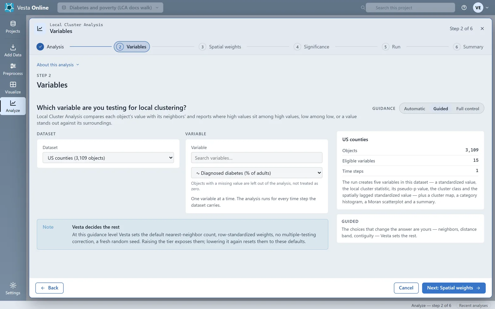
The neighbors
Section titled “The neighbors”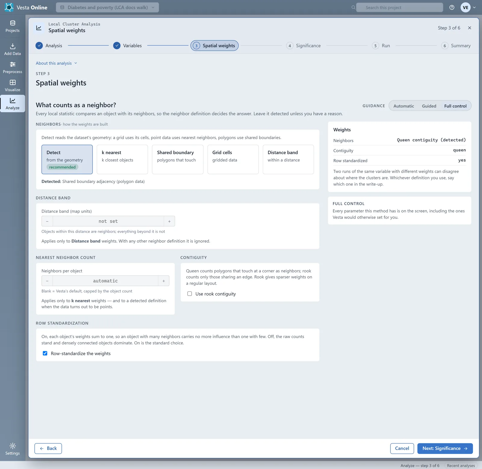
The significance
Section titled “The significance”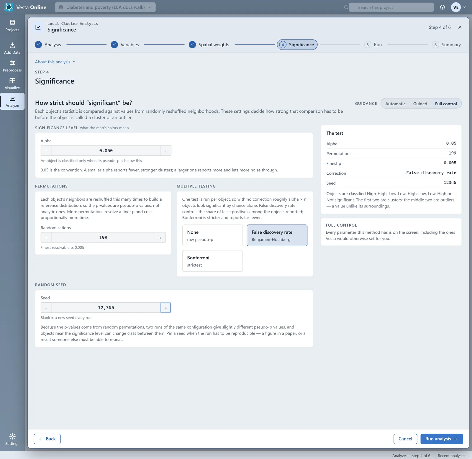
The summary
Section titled “The summary”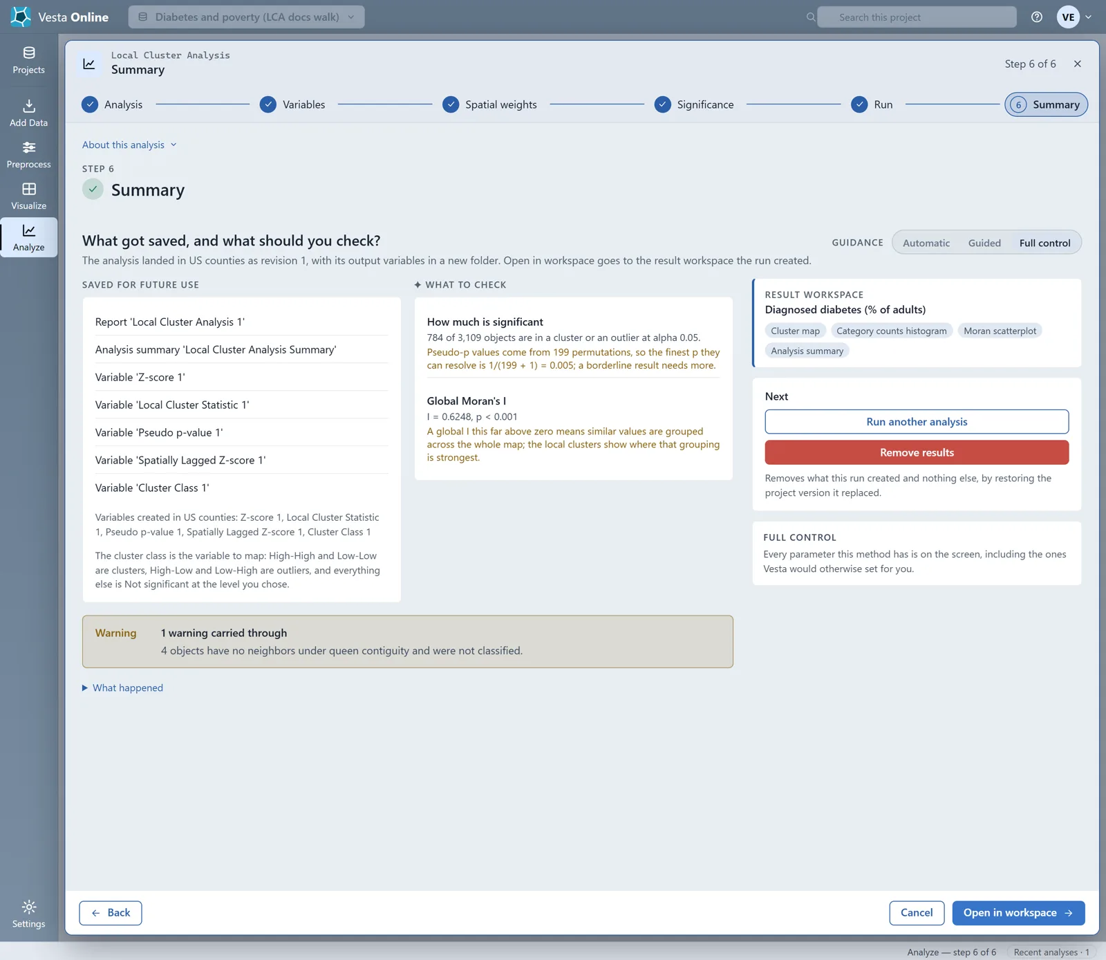
The run adds five variables to the dataset: a standardized value, the local cluster statistic, its pseudo-p value, the cluster class and the spatially lagged standardized value. The cluster class is the one to map. The Summary also carries a warning from this run: 4 objects have no neighbors under queen contiguity and were not classified.
The result
Section titled “The result”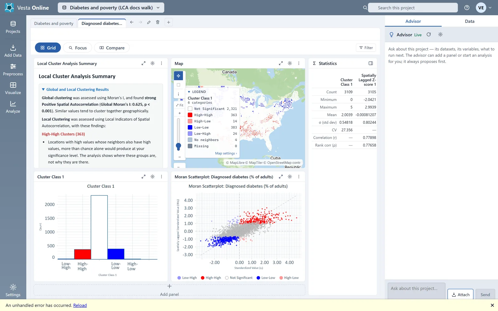
Reading the result
Section titled “Reading the result”In this run, with False discovery rate and alpha 0.05, 784 of the 3,109 counties are in a cluster or an outlier: 363 High-High, 383 Low-Low, 14 High-Low and 24 Low-High. Another 2,321 are Not Significant, and 4 counties are islands (Dukes, Nantucket, Richmond and San Juan) that share no boundary with another county, so under shared-boundary weights they have no neighbors and are not tested. This run gives them the class No neighbors, not Missing. The 784, the 2,321 and these 4 account for all 3,109. Global Moran’s I is 0.6248 (p < 0.001), so similar values are grouped across the whole map; the local clusters show where that grouping is strongest. The classes mean this:
| Class | Meaning |
|---|---|
| High-High | A high value among neighbors that are also high: a hot spot. |
| Low-Low | A low value among neighbors that are also low: a cold spot. |
| High-Low | A high value among lower neighbors: an outlier. |
| Low-High | A low value among higher neighbors: an outlier. |
| Not Significant | No clear local pattern at the alpha you chose. |
| No neighbors | A county with a value but no neighbors under the weights you chose, such as an island. It is not tested and not classified. |
The first two are clusters; the middle two are outliers.
Where next
Section titled “Where next”- Your first run, with the defaults: Quickstart.
- Model what drives the pattern: Regression and GWR.
- Bring in your own data: Importing data.
Not sure which method fits your question? When the Advisor is turned on, you can describe your question on the Analysis step and let the Advisor suggest one. The Advisor is an optional AI-assisted guided workflow; see Using the Advisor.