Regression and GWR

Regression asks how much one variable is explained by others. Geographically weighted regression (GWR) asks the same question at every location, so the relationship can change across the map. This walk-through runs both on one pair of county variables, diagnosed diabetes (percent of adults) explained by the poverty rate (percent of people), for the 3,109 counties of the Diabetes and poverty sample. Every step below was run on Vesta Online, on a copy of that sample project; the screenshots come from that run.

The eleven steps

1. 1Open a project that holds your dataOpen the Projects page, select your project and choose Open Project. You need a dataset with a numeric response and at least one numeric predictor; the walk used a copy of the Diabetes and poverty sample, so the sample itself stays unchanged.
2. 2Choose the response and the predictorChoose Analyze, then Explain a relationship, then Regression (OLS / logistic). On Variables, pick the dataset (US counties), set Dependent variable to Diagnosed diabetes (% of adults), and under Explanatory variables add Poverty rate (% of people).
3. 3Save the residualsChoose Next: Options and tick Save the residuals. Leave time as a predictor off, and the seed alone.
4. 4Run the regressionChoose Run analysis and stay on the page. When the Summary step says what was saved, the run is done.
5. 5Open the regression resultChoose Open in workspace. The result workspace shows the Regression Summary, an observed versus estimated scatterplot, an Estimated Mean map and a Standard Error map.
6. 6Choose the same variables for GWRChoose Analyze, then Explain a relationship, then Geographically weighted regression. On Variables pick the same dataset, response and predictor.
7. 7Review the bandwidth searchChoose Next: Bandwidth. The bandwidth is not entered; Vesta searches for it. At the default Guided level it uses a Gaussian kernel and 35 candidate widths.
8. 8Keep the coefficient surfacesChoose Next: Options. Save the local coefficient surfaces is ticked by default; leave it ticked, because the surfaces are the reason to run GWR.
9. 9Run the GWRChoose Run analysis. A GWR refits the model at every candidate width, so it can take longer than the regression; stay on the page. The Summary step lists what was saved.
10. 10Open the GWR coefficient surfacesChoose Open in workspace, the button at the bottom right of the Summary step. It opens the first of the two result workspaces, the Coefficient surface browser: a map of the local coefficient for each predictor.
11. 11Read the GWR summaryChoose the workspace tab named after the response with a 1, the second result workspace. It holds the GWR Analysis Summary, the predicted map, an observed versus predicted scatterplot and a Local R-squared map.

What you should see

Choosing the variables

Variables

One response and one predictor. The card on the right reads least squares because the response is continuous.

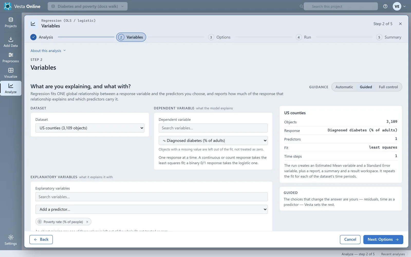
The response can be continuous, a count or binary. A continuous or count response takes the least-squares fit. Objects with a missing value are left out of the fit, not treated as zero.

NoteA binary 0/1 response selects logistic regression instead. The run then reports accuracy, an ROC curve and the area under it rather than R-squared, and writes a predicted label and a probability instead of an estimated mean. This article did not walk the logistic arm.

Options

Options

Saving the residuals adds a third variable to the two the regression always writes.

The regression always saves an Estimated Mean and a Standard Error for each county. Saving the residuals adds one more variable: the observed value minus the predicted one. Positive residuals mean the fit under-predicted there, negative that it over-predicted. Residuals are not saved unless you tick the box.

The summary

Summary

The Summary step lists what was saved and three things to check.

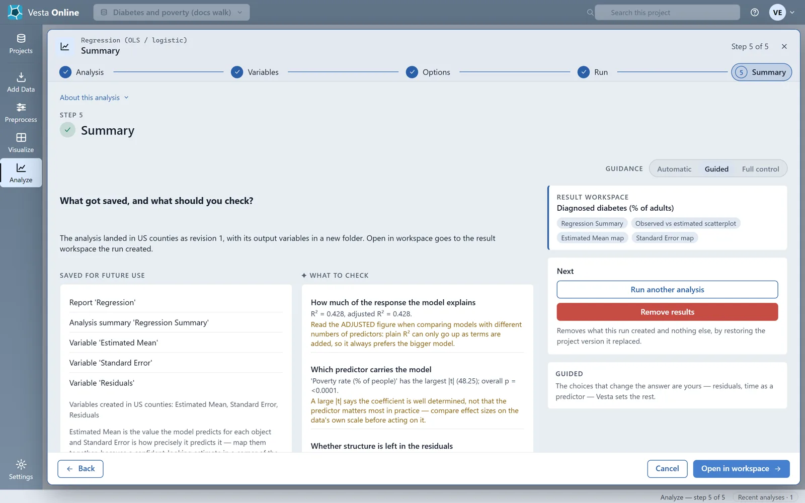
For this run R-squared is 0.428 (adjusted 0.428), and poverty has the largest absolute t value, 48.25. Read the adjusted figure when you compare models with different numbers of predictors. A large t says the coefficient is well determined, not that the predictor matters most in practice. The third check is the residual Moran’s I, 0.351. Near zero is what you want; a clearly positive value means neighboring residuals still agree, so the model is missing something spatial.

The regression result

Result workspace

The written summary, the scatterplot and the two maps.

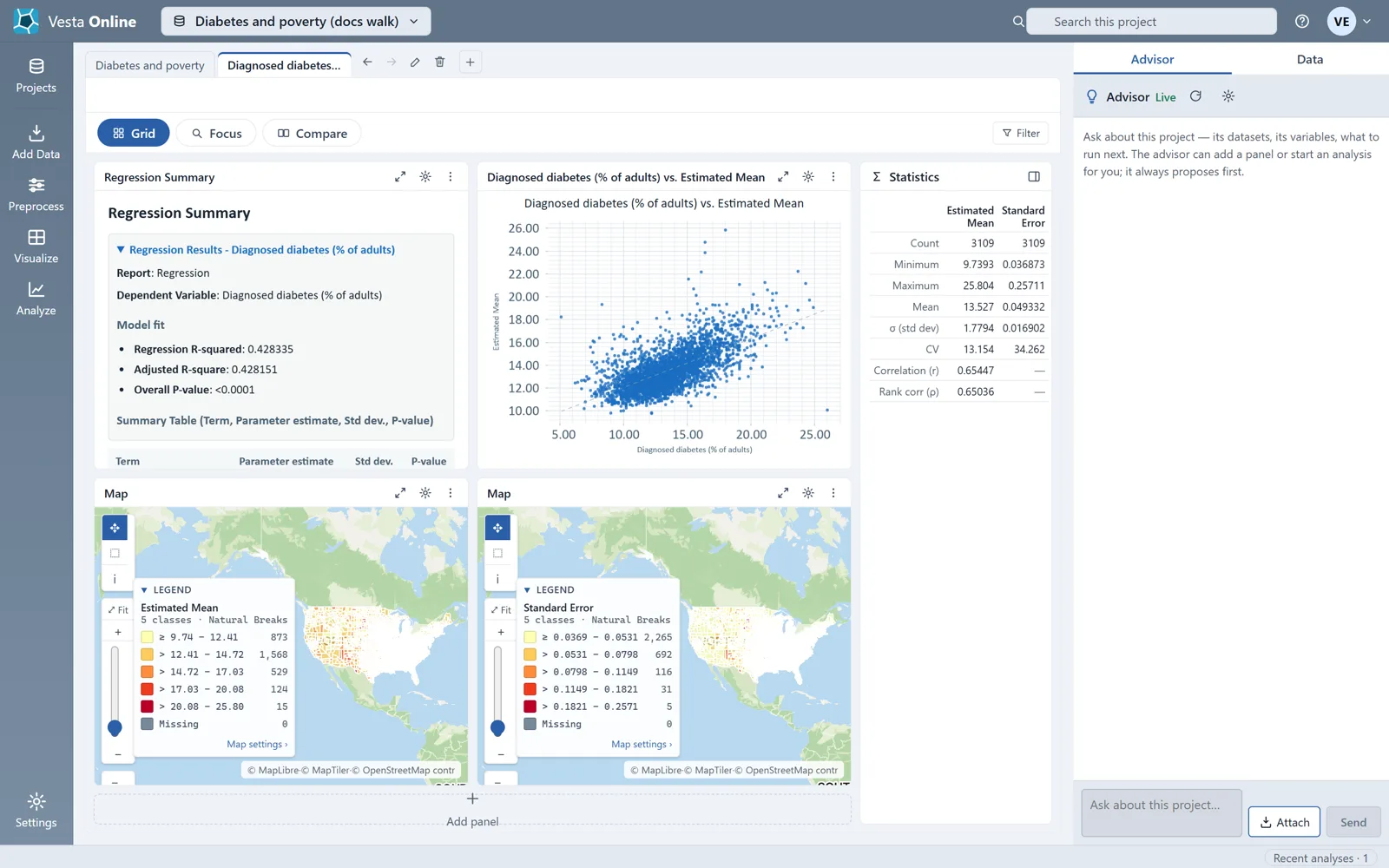
Map the Estimated Mean and the Standard Error together: a confident-looking estimate in a place with a large standard error is the one to distrust. Because the residual Moran’s I is clearly positive, one global slope leaves a spatial pattern behind. That is a reason to try GWR.

The bandwidth

Bandwidth

The bandwidth is optimized by search, not entered.

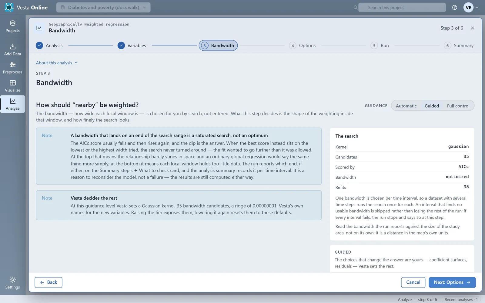
GWR fits a separate regression at every location, using only the observations near it, and the bandwidth says how wide that neighborhood is. Vesta uses a fixed-distance bandwidth, the same distance everywhere, chosen by AICc. The step also warns about a bandwidth that lands on either end of the search range: that means the search never turned around, which is a reason to reconsider the model rather than a failure. The run reports which end, if either, on the Summary step.

Options

Options

Coefficient surfaces are on by default; the residual surface is off.

With the surfaces on, the run saves two variables for every column of the design matrix, a local beta coefficient and a local t statistic beside it, and the intercept counts as a column. One predictor means at least four extra variables, and here seven new variables in all with the predicted value, local R-squared and local variance. Saving the residual surface adds one more.

The GWR summary

Summary

A GWR run creates two result workspaces.

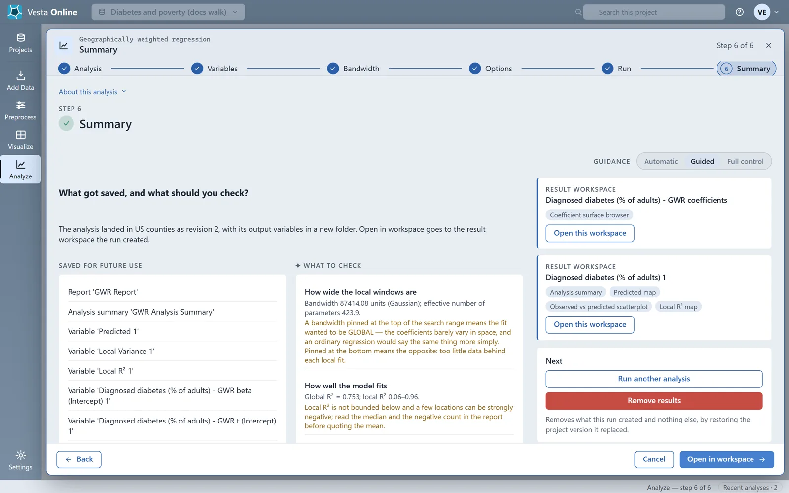
The Summary step reports the bandwidth (87414.08 units here, a distance in the map’s own units), the global R-squared (0.753 here), the range of the local R-squared (0.06 to 0.96) and the residual Moran’s I, which is 0.009 here against 0.351 for the single regression. The near-zero value suggests that the local models have absorbed the spatial structure. This is a comparison of two runs on one dataset, not a test of which model is right.

The coefficient surfaces

Coefficient surface browser

The local coefficient for poverty rate, county by county.

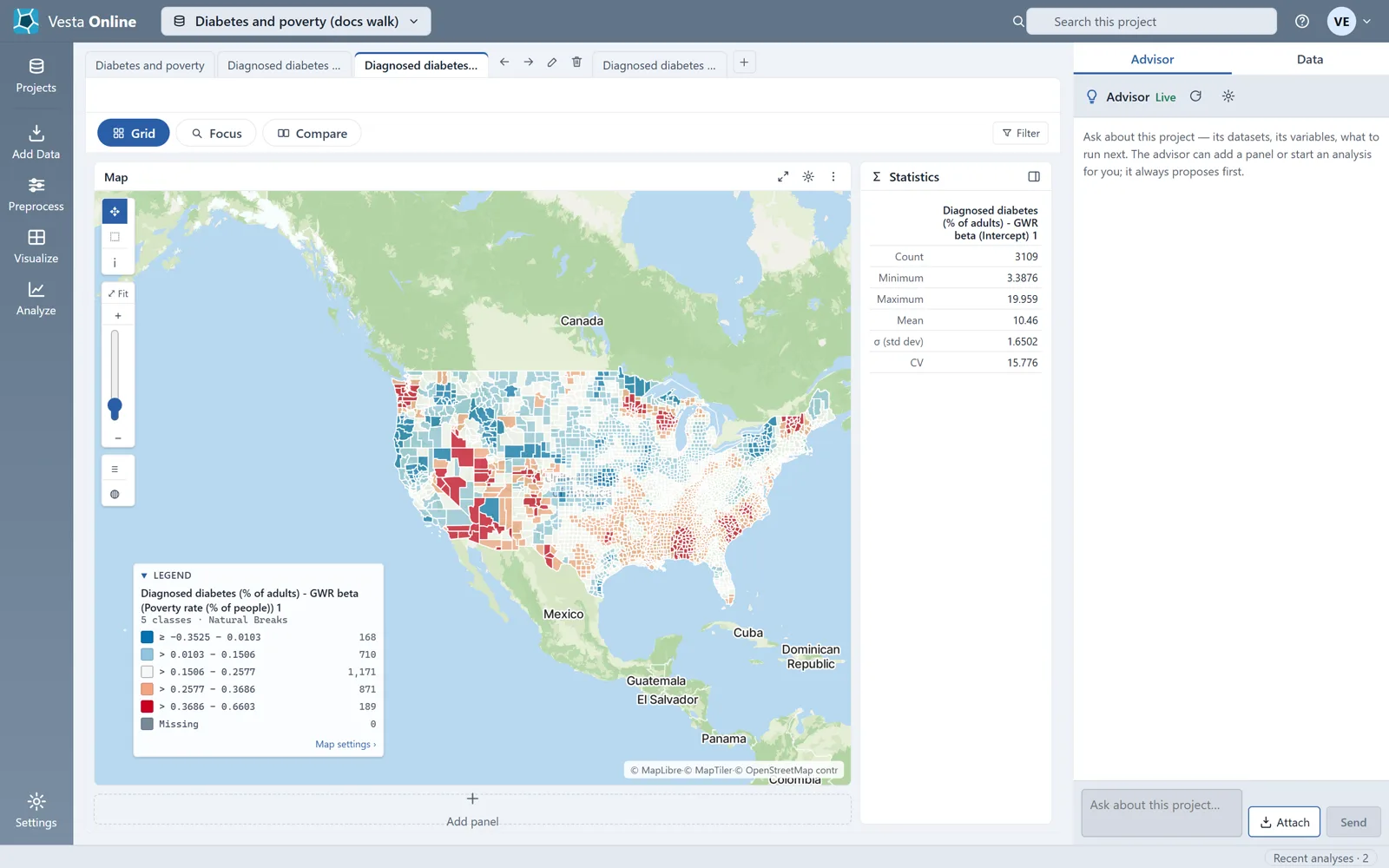
This is what a global regression cannot give you: the relationship between poverty and diabetes is stronger in some regions than in others. Every county shows a number, including those where the local t says the coefficient is indistinguishable from zero, so check the local t before reading a sign off the map.

The GWR workspace

Result workspace

The written GWR summary with the predicted and local R-squared maps.

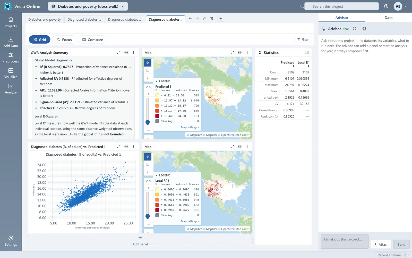
Local R-squared is not bounded below by 0: a location scores below zero when its local model predicts worse than the local weighted average. Read the median, not only the mean, and inspect the Local R-squared map to see where the model works and where it struggles. Correlated predictors make local coefficient surfaces unstable, which matters once you add a second predictor.

Limits

NoteEach analysis fits one response at a time. An object missing any one of the chosen values is left out of the whole fit, not treated as zero. A categorical predictor is one-hot encoded, so it becomes several columns, each with a coefficient of its own.

NoteAn analysis of yours must finish before the next one starts. If another run of your account is still going, the Run step says Another analysis of yours is still running; wait for it to finish, then choose Try again.

NoteAll metrics in a logistic summary are in-sample, so they may overestimate performance on new data. Statistics from either method describe the fitted sample; read them as description, not as proof of cause.

Where next

• Find where values cluster before modeling them: Local cluster analysis.
• Get started with a first project: Quickstart.
• Estimate values between sample points: Kriging.

Not sure which method fits your question? When the Advisor is turned on, you can describe your question on the Analysis step and let the Advisor suggest one. The Advisor is an optional AI-assisted guided workflow; see Using the Advisor.